Not `mtcars` AGAIN

Published

Last modified on March 15, 2025 15:44:30 Eastern Daylight Time

Crediting the materials

The majority of the material in the first part of this document is taken from the free online course at https://supervised-ml-course.netlify.app/ written by Julia Silge.

In this first case study, you will predict fuel efficiency from a US Department of Energy data set for real cars of today.

In this case study, you will predict the fuel efficiency ⛽ of modern cars from characteristics of these cars, like transmission and engine displacement. Fuel efficiency is a numeric value that ranges smoothly from about 15 to 40 miles per gallon. To predict fuel efficiency you will build a Regression model.

Visualize the fuel efficiency distribution

The first step before you start modeling is to explore your data. In this course we’ll practice using tidyverse functions for exploratory data analysis. Start off this case study by examining your data set and visualizing the distribution of fuel efficiency. The ggplot2 package, with functions like ggplot() and geom_histogram(), is included in the tidyverse. The tidyverse metapackage is loaded for you, so you can use readr and ggplot2.

library(tidyverse)
cars2018 <- read_csv("../Data/cars2018.csv")

Take a look at the cars2018 object using glimpse().

# Print the cars2018 object
glimpse(cars2018)

Rows: 1,144
Columns: 15
$ model                   <chr> "Acura NSX", "ALFA ROMEO 4C", "Audi R8 AWD", "…
$ model_index             <dbl> 57, 410, 65, 71, 66, 72, 46, 488, 38, 278, 223…
$ displacement            <dbl> 3.5, 1.8, 5.2, 5.2, 5.2, 5.2, 2.0, 3.0, 8.0, 6…
$ cylinders               <dbl> 6, 4, 10, 10, 10, 10, 4, 6, 16, 8, 8, 8, 8, 8,…
$ gears                   <dbl> 9, 6, 7, 7, 7, 7, 6, 7, 7, 8, 8, 7, 7, 7, 7, 7…
$ transmission            <chr> "Manual", "Manual", "Manual", "Manual", "Manua…
$ mpg                     <dbl> 21, 28, 17, 18, 17, 18, 26, 20, 11, 18, 16, 18…
$ aspiration              <chr> "Turbocharged/Supercharged", "Turbocharged/Sup…
$ lockup_torque_converter <chr> "Y", "Y", "Y", "Y", "Y", "Y", "Y", "N", "Y", "…
$ drive                   <chr> "All Wheel Drive", "2-Wheel Drive, Rear", "All…
$ max_ethanol             <dbl> 10, 10, 15, 15, 15, 15, 15, 10, 15, 10, 10, 10…
$ recommended_fuel        <chr> "Premium Unleaded Required", "Premium Unleaded…
$ intake_valves_per_cyl   <dbl> 2, 2, 2, 2, 2, 2, 2, 2, 2, 1, 1, 1, 1, 2, 2, 2…
$ exhaust_valves_per_cyl  <dbl> 2, 2, 2, 2, 2, 2, 2, 2, 2, 1, 1, 1, 1, 2, 2, 2…
$ fuel_injection          <chr> "Direct ignition", "Direct ignition", "Direct …

Use the appropriate column from cars2018 in the call to aes() so you can plot a histogram of fuel efficiency (miles per gallon, mpg). Set the correct x and y labels.

# Plot the histogram
ggplot(cars2018, aes(x = mpg)) +
  geom_histogram(bins = 25, color = "black", fill = "red") +
  labs(x = "Fuel efficiency (mpg)",
       y = "Number of cars") + 
  theme_bw()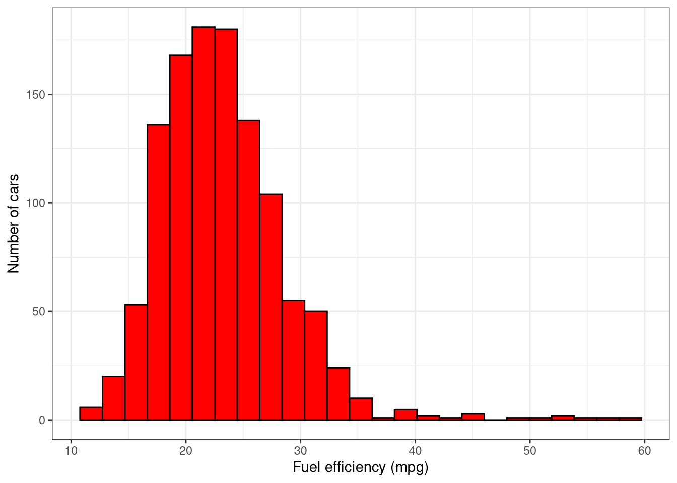

# Consider using log10(mpg) instead of mpg
cars2018 <- cars2018 |> 
  mutate(log_mpg = log(mpg))
ggplot(cars2018, aes(x = log_mpg)) +
  geom_histogram(bins = 15, color = "black", fill = "red") +
  labs(x = "Fuel efficiency (log_mpg)",
       y = "Number of cars") + 
  theme_bw()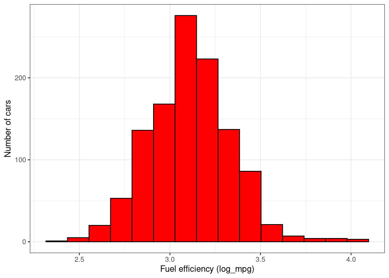

Build a simple linear model

Before embarking on more complex machine learning models, it’s a good idea to build the simplest possible model to get an idea of what is going on. In this case, that means fitting a simple linear model using base R’s lm() function.

Instructions

Use select() to deselect the two columns model and model_index from cars2018; these columns tell us the individual identifiers for each car and it would not make sense to include them in modeling. Store the results in car_vars.

# Deselect the 2 columns to create cars_vars
car_vars <- cars2018 |> 
    select(-model, -model_index)

Fit mpg as the predicted quantity, explained by all the predictors, i.e., . in the R formula input to lm(). Store the linear model object in fit_all. (You may have noticed the log distribution of MPG in the last exercise, but don’t worry about fitting the logarithm of fuel efficiency yet.)

# Fit a linear model
fit_all <- lm(mpg ~ . - log_mpg, data = car_vars)

Print the summary() of the modelfit_all`.

# Print the summary of the model
summary(fit_all)


Call:
lm(formula = mpg ~ . - log_mpg, data = car_vars)

Residuals:
    Min      1Q  Median      3Q     Max 
-8.5261 -1.6473 -0.1096  1.3572 26.5045 

Coefficients:
                                              Estimate Std. Error t value
(Intercept)                                  44.539519   1.176283  37.865
displacement                                 -3.786147   0.264845 -14.296
cylinders                                     0.520284   0.161802   3.216
gears                                         0.157674   0.069984   2.253
transmissionCVT                               4.877637   0.404051  12.072
transmissionManual                           -1.074608   0.366075  -2.935
aspirationTurbocharged/Supercharged          -2.190248   0.267559  -8.186
lockup_torque_converterY                     -2.624494   0.381252  -6.884
drive2-Wheel Drive, Rear                     -2.676716   0.291044  -9.197
drive4-Wheel Drive                           -3.397532   0.335147 -10.137
driveAll Wheel Drive                         -2.941084   0.257174 -11.436
max_ethanol                                  -0.007377   0.005898  -1.251
recommended_fuelPremium Unleaded Required    -0.403935   0.262413  -1.539
recommended_fuelRegular Unleaded Recommended -0.996343   0.272495  -3.656
intake_valves_per_cyl                        -1.446107   1.620575  -0.892
exhaust_valves_per_cyl                       -2.469747   1.547748  -1.596
fuel_injectionMultipoint/sequential ignition -0.658428   0.243819  -2.700
                                             Pr(>|t|)    
(Intercept)                                   < 2e-16 ***
displacement                                  < 2e-16 ***
cylinders                                    0.001339 ** 
gears                                        0.024450 *  
transmissionCVT                               < 2e-16 ***
transmissionManual                           0.003398 ** 
aspirationTurbocharged/Supercharged          7.24e-16 ***
lockup_torque_converterY                     9.65e-12 ***
drive2-Wheel Drive, Rear                      < 2e-16 ***
drive4-Wheel Drive                            < 2e-16 ***
driveAll Wheel Drive                          < 2e-16 ***
max_ethanol                                  0.211265    
recommended_fuelPremium Unleaded Required    0.124010    
recommended_fuelRegular Unleaded Recommended 0.000268 ***
intake_valves_per_cyl                        0.372400    
exhaust_valves_per_cyl                       0.110835    
fuel_injectionMultipoint/sequential ignition 0.007028 ** 
---
Signif. codes:  0 '***' 0.001 '**' 0.01 '*' 0.05 '.' 0.1 ' ' 1

Residual standard error: 2.916 on 1127 degrees of freedom
Multiple R-squared:  0.7314,    Adjusted R-squared:  0.7276 
F-statistic: 191.8 on 16 and 1127 DF,  p-value: < 2.2e-16

# Better yet
broom::tidy(fit_all) |> 
  knitr::kable()

term	estimate	std.error	statistic	p.value
(Intercept)	44.5395187	1.1762833	37.8646201	0.0000000
displacement	-3.7861470	0.2648450	-14.2957074	0.0000000
cylinders	0.5202836	0.1618015	3.2155668	0.0013389
gears	0.1576744	0.0699836	2.2530183	0.0244497
transmissionCVT	4.8776374	0.4040514	12.0718250	0.0000000
transmissionManual	-1.0746077	0.3660748	-2.9354869	0.0033978
aspirationTurbocharged/Supercharged	-2.1902481	0.2675589	-8.1860399	0.0000000
lockup_torque_converterY	-2.6244942	0.3812516	-6.8838898	0.0000000
drive2-Wheel Drive, Rear	-2.6767162	0.2910442	-9.1969408	0.0000000
drive4-Wheel Drive	-3.3975319	0.3351470	-10.1374366	0.0000000
driveAll Wheel Drive	-2.9410836	0.2571744	-11.4361445	0.0000000
max_ethanol	-0.0073774	0.0058981	-1.2508063	0.2112648
recommended_fuelPremium Unleaded Required	-0.4039345	0.2624128	-1.5393093	0.1240095
recommended_fuelRegular Unleaded Recommended	-0.9963428	0.2724946	-3.6563764	0.0002676
intake_valves_per_cyl	-1.4461074	1.6205748	-0.8923423	0.3724000
exhaust_valves_per_cyl	-2.4697466	1.5477481	-1.5957032	0.1108354
fuel_injectionMultipoint/sequential ignition	-0.6584282	0.2438186	-2.7004839	0.0070276

# and
broom::glance(fit_all) |> 
  knitr::kable()

r.squared	adj.r.squared	sigma	statistic	p.value	df	logLik	AIC	BIC	deviance	df.residual	nobs
0.7313934	0.72758	2.915576	191.7955	0	16	-2838.859	5713.718	5804.479	9580.16	1127	1144

You just performed some exploratory data analysis and built a simple linear model using base R’s lm() function.

Getting started with `tidymodels`

Training and testing data

Training models based on all of your data at once is typically not a good choice. 🚫 Instead, you can create subsets of your data that you use for different purposes, such as training your model and then testing your model.

Creating training/testing splits reduces overfitting. When you evaluate your model on data that it was not trained on, you get a better estimate of how it will perform on new data.

Instructions

Load the tidymodels metapackage, which also includes dplyr for data manipulation.

# Load tidymodels
library(tidymodels)

Create a data split that divides the original data into 80%/20% sections and (roughly) evenly divides the partitions between the different types of transmission. Assign the 80% partition to car_train and the 20% partition to car_test.

# Split the data into training and test sets
set.seed(1234)
car_split <- car_vars |> 
    select(-mpg) |> 
    initial_split(prop = 0.8, strata = transmission)

car_train <- training(car_split)
car_test <- testing(car_split)

glimpse(car_train)

Rows: 915
Columns: 13
$ displacement            <dbl> 6.2, 6.2, 1.4, 2.0, 2.0, 3.0, 3.0, 3.0, 3.0, 3…
$ cylinders               <dbl> 8, 8, 4, 4, 4, 6, 6, 6, 6, 6, 4, 8, 6, 8, 6, 6…
$ gears                   <dbl> 8, 8, 6, 8, 8, 8, 8, 8, 8, 8, 6, 7, 9, 9, 7, 7…
$ transmission            <chr> "Automatic", "Automatic", "Automatic", "Automa…
$ aspiration              <chr> "Naturally Aspirated", "Turbocharged/Superchar…
$ lockup_torque_converter <chr> "Y", "Y", "Y", "Y", "Y", "Y", "Y", "Y", "Y", "…
$ drive                   <chr> "2-Wheel Drive, Rear", "2-Wheel Drive, Rear", …
$ max_ethanol             <dbl> 10, 10, 10, 15, 15, 15, 15, 15, 15, 15, 10, 10…
$ recommended_fuel        <chr> "Premium Unleaded Required", "Premium Unleaded…
$ intake_valves_per_cyl   <dbl> 1, 1, 2, 2, 2, 2, 2, 2, 2, 2, 2, 2, 2, 2, 2, 2…
$ exhaust_valves_per_cyl  <dbl> 1, 1, 2, 2, 2, 2, 2, 2, 2, 2, 2, 2, 2, 2, 2, 2…
$ fuel_injection          <chr> "Direct ignition", "Direct ignition", "Multipo…
$ log_mpg                 <dbl> 2.890372, 2.772589, 3.367296, 3.258097, 3.2580…

glimpse(car_test)

Rows: 229
Columns: 13
$ displacement            <dbl> 8.0, 6.2, 3.9, 6.5, 3.0, 5.0, 5.0, 2.0, 4.0, 4…
$ cylinders               <dbl> 16, 8, 8, 12, 6, 8, 8, 4, 8, 8, 12, 6, 4, 4, 6…
$ gears                   <dbl> 7, 7, 7, 7, 8, 8, 8, 6, 7, 7, 7, 9, 9, 6, 7, 7…
$ transmission            <chr> "Manual", "Manual", "Manual", "Manual", "Autom…
$ aspiration              <chr> "Turbocharged/Supercharged", "Naturally Aspira…
$ lockup_torque_converter <chr> "Y", "N", "N", "N", "Y", "Y", "Y", "N", "Y", "…
$ drive                   <chr> "All Wheel Drive", "2-Wheel Drive, Rear", "2-W…
$ max_ethanol             <dbl> 15, 10, 10, 10, 15, 15, 15, 10, 10, 10, 10, 10…
$ recommended_fuel        <chr> "Premium Unleaded Required", "Premium Unleaded…
$ intake_valves_per_cyl   <dbl> 2, 1, 2, 2, 2, 2, 2, 2, 2, 2, 2, 2, 2, 2, 2, 2…
$ exhaust_valves_per_cyl  <dbl> 2, 1, 2, 2, 2, 2, 2, 2, 2, 2, 1, 2, 2, 2, 2, 2…
$ fuel_injection          <chr> "Multipoint/sequential ignition", "Direct igni…
$ log_mpg                 <dbl> 2.397895, 2.944439, 2.890372, 2.564949, 3.1354…

Train models with `tidymodels`

Now that your car_train data is ready, you can fit a set of models with tidymodels. When we model data, we deal with model type (such as linear regression or random forest), mode (regression or classification), and model engine (how the models are actually fit). In tidymodels, we capture that modeling information in a model specification, so setting up your model specification can be a good place to start. In these exercises, fit one linear regression model and one random forest model, without any resampling of your data.

Instructions

Fit a basic linear regression model to your car_train data. (Notice that we are fitting to log(mpg) since the fuel efficiency had a log normal distribution.)

# Build a linear regression model specification
lm_spec <- linear_reg() |> 
    set_engine("lm")

# Train a linear regression model
fit_lm <- lm_spec |> 
    fit(log_mpg ~ ., data = car_train)

# Print the model object
broom::tidy(fit_lm) |> 
  knitr::kable()

term	estimate	std.error	statistic	p.value
(Intercept)	4.0058963	0.0456229	87.804508	0.0000000
displacement	-0.1591673	0.0101472	-15.685813	0.0000000
cylinders	0.0092052	0.0062212	1.479654	0.1393162
gears	0.0115071	0.0027283	4.217720	0.0000272
transmissionCVT	0.1612901	0.0158513	10.175223	0.0000000
transmissionManual	-0.0274861	0.0142674	-1.926491	0.0543584
aspirationTurbocharged/Supercharged	-0.0984454	0.0104909	-9.383906	0.0000000
lockup_torque_converterY	-0.0740208	0.0149250	-4.959510	0.0000008
drive2-Wheel Drive, Rear	-0.0855545	0.0113160	-7.560472	0.0000000
drive4-Wheel Drive	-0.1273189	0.0130941	-9.723398	0.0000000
driveAll Wheel Drive	-0.1058523	0.0102251	-10.352212	0.0000000
max_ethanol	-0.0002975	0.0002248	-1.323348	0.1860565
recommended_fuelPremium Unleaded Required	-0.0163239	0.0102396	-1.594199	0.1112432
recommended_fuelRegular Unleaded Recommended	-0.0434804	0.0107403	-4.048329	0.0000560
intake_valves_per_cyl	-0.0788364	0.0647617	-1.217331	0.2237981
exhaust_valves_per_cyl	-0.0831906	0.0619699	-1.342435	0.1797942
fuel_injectionMultipoint/sequential ignition	-0.0331051	0.0094613	-3.498991	0.0004900

# and
broom::glance(fit_lm) |> 
  knitr::kable()

r.squared	adj.r.squared	sigma	statistic	p.value	df	logLik	AIC	BIC	deviance	df.residual	nobs
0.8061189	0.8026644	0.1014553	233.3565	0	16	803.8961	-1571.792	-1485.052	9.243282	898	915

Fit a random forest model to your car_train data.

# Build a random forest model specification
rf_spec <- rand_forest() |> 
    set_engine("ranger", importance = "impurity") |> 
    set_mode("regression")

# Train a random forest model
fit_rf <- rf_spec |> 
    fit(log_mpg ~ ., data = car_train)

# Print the model object
fit_rf

parsnip model object

Ranger result

Call:
 ranger::ranger(x = maybe_data_frame(x), y = y, importance = ~"impurity",      num.threads = 1, verbose = FALSE, seed = sample.int(10^5,          1)) 

Type:                             Regression 
Number of trees:                  500 
Sample size:                      915 
Number of independent variables:  12 
Mtry:                             3 
Target node size:                 5 
Variable importance mode:         impurity 
Splitrule:                        variance 
OOB prediction error (MSE):       0.007038903 
R squared (OOB):                  0.8650538

vip::vip(fit_rf) +
  theme_bw()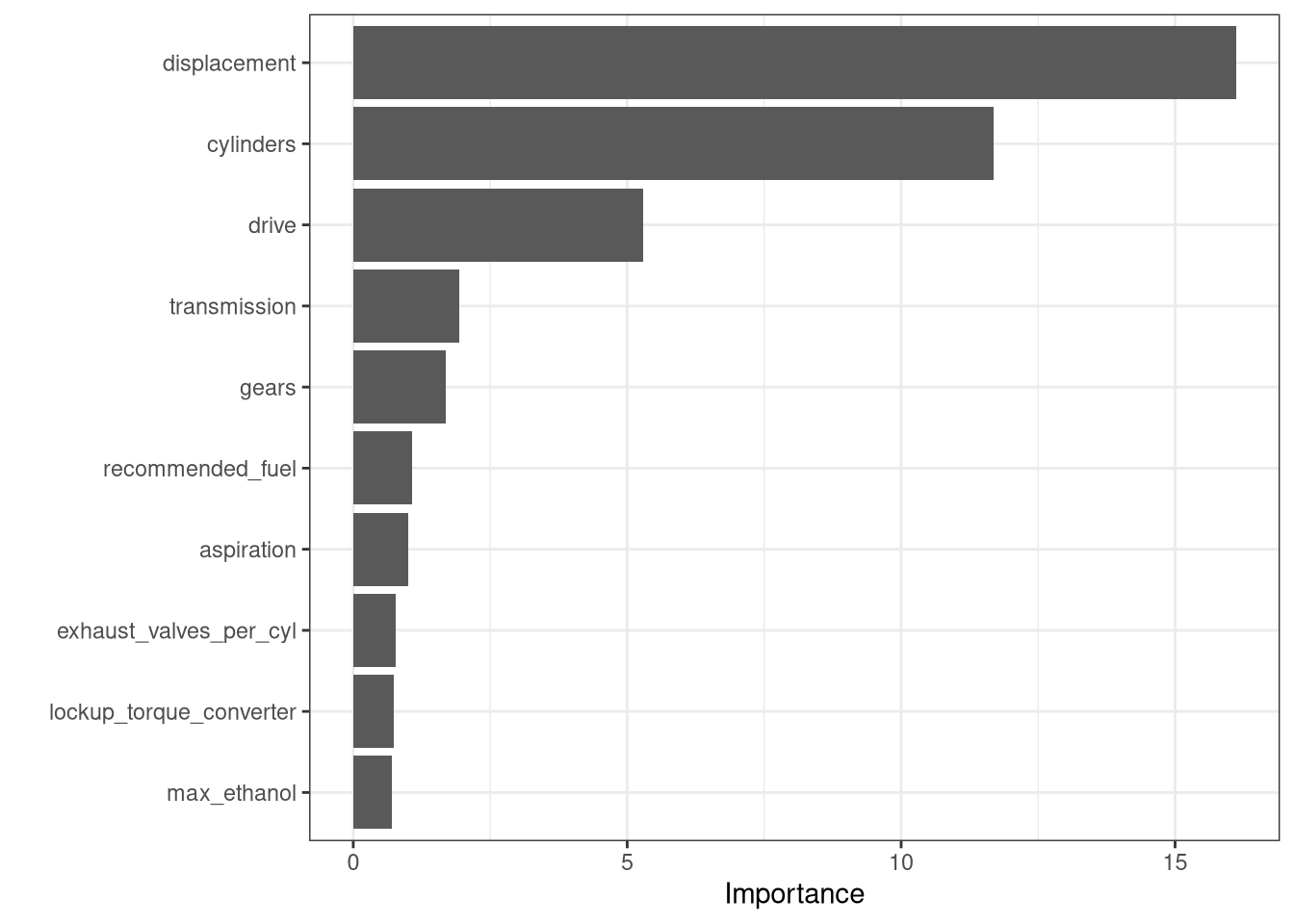

Evaluate model performance

The fit_lm and fit_rf models you just trained are in your environment. It’s time to see how they did! 🤩 How are we doing do this, though?! 🤔 There are several things to consider, including both what metrics and what data to use.

For regression models, we will focus on evaluating using the root mean squared error metric. This quantity is measured in the same units as the original data (log of miles per gallon, in our case). Lower values indicate a better fit to the data. It’s not too hard to calculate root mean squared error manually, but the yardstick package offers convenient functions for this and many other model performance metrics.

Instructions

Note: The yardstick package is loaded since it is one of the packages in tidyverse.

Create new columns for model predictions from each of the models you have trained, first linear regression and then random forest.

# Create the new columns
results <- car_train |> 
    bind_cols(predict(fit_lm, car_train) |> 
                  rename(.pred_lm = .pred)) |> 
    bind_cols(predict(fit_rf, car_train) |> 
                  rename(.pred_rf = .pred)) |> 
    relocate(log_mpg, .pred_lm, .pred_rf, .before = displacement)
head(results) |> 
  knitr::kable()

log_mpg	.pred_lm	.pred_rf	displacement	cylinders	gears	transmission	aspiration	lockup_torque_converter	drive	max_ethanol	recommended_fuel	intake_valves_per_cyl	exhaust_valves_per_cyl	fuel_injection
2.890372	2.843856	2.868826	6.2	8	8	Automatic	Naturally Aspirated	Y	2-Wheel Drive, Rear	10	Premium Unleaded Required	1	1	Direct ignition
2.772589	2.745411	2.821072	6.2	8	8	Automatic	Turbocharged/Supercharged	Y	2-Wheel Drive, Rear	10	Premium Unleaded Required	1	1	Direct ignition
3.367296	3.270770	3.317601	1.4	4	6	Automatic	Turbocharged/Supercharged	Y	2-Wheel Drive, Rear	10	Premium Unleaded Recommended	2	2	Multipoint/sequential ignition
3.258097	3.229902	3.254968	2.0	4	8	Automatic	Turbocharged/Supercharged	Y	2-Wheel Drive, Rear	15	Premium Unleaded Recommended	2	2	Direct ignition
3.258097	3.229902	3.254968	2.0	4	8	Automatic	Turbocharged/Supercharged	Y	2-Wheel Drive, Rear	15	Premium Unleaded Recommended	2	2	Direct ignition
3.135494	3.089145	3.089431	3.0	6	8	Automatic	Turbocharged/Supercharged	Y	2-Wheel Drive, Rear	15	Premium Unleaded Recommended	2	2	Direct ignition

Evaluate the performance of these models using metrics() by specifying the column that contains the real fuel efficiency.

# Evaluate the performance
metrics(results, truth = log_mpg, estimate = .pred_lm) |> 
  knitr::kable()

.metric	.estimator	.estimate
rmse	standard	0.1005084
rsq	standard	0.8061189
mae	standard	0.0746879

metrics(results, truth = log_mpg, estimate = .pred_rf) |> 
  knitr::kable()

.metric	.estimator	.estimate
rmse	standard	0.0681861
rsq	standard	0.9140019
mae	standard	0.0493565

Use the testing data

“But wait!” you say, because you have been paying attention. 🤔 “That is how these models perform on the training data, the data that we used to build these models in the first place.” This is not a good idea because when you evaluate on the same data you used to train a model, the performance you estimate is too optimistic.

Let’s evaluate how these simple models perform on the testing data instead.

# Create the new columns
results <- car_test  |> 
    bind_cols(predict(fit_lm, car_test)  |> 
                  rename(.pred_lm = .pred))  |> 
    bind_cols(predict(fit_rf, car_test)  |> 
                  rename(.pred_rf = .pred)) |> 
    relocate(log_mpg, .pred_lm, .pred_rf, .before = displacement)

# Evaluate the performance
metrics(results, truth = log_mpg, estimate = .pred_lm) |> 
  knitr::kable()

.metric	.estimator	.estimate
rmse	standard	0.0969079
rsq	standard	0.8036351
mae	standard	0.0727383

metrics(results, truth = log_mpg, estimate = .pred_rf) |> 
  knitr::kable()

.metric	.estimator	.estimate
rmse	standard	0.0791940
rsq	standard	0.8743060
mae	standard	0.0583998

You just trained models one time on the whole training set and then evaluated them on the testing set. Statisticians have come up with a slew of approaches to evaluate models in better ways than this; many important ones fall under the category of resampling.

The idea of resampling is to create simulated data sets that can be used to estimate the performance of your model, say, because you want to compare models. You can create these resampled data sets instead of using either your training set (which can give overly optimistic results, especially for powerful ML algorithms) or your testing set (which is extremely valuable and can only be used once or at most twice).

The first resampling approach we’re going to try in this course is called the bootstrap. Bootstrap resampling means drawing with replacement from our original dataset and then fitting on that dataset.

Let’s think about…cars! 🚗🚌🚙🚕

Bootstrap resampling

In the last set of exercises, you trained linear regression and random forest models without any resampling. Resampling can help us evaluate our machine learning models more accurately.

Let’s try bootstrap resampling, which means creating data sets the same size as the original one by randomly drawing with replacement from the original. In tidymodels, the default behavior for bootstrapping is 25 resamplings, but you can change this using the times argument in bootstraps() if desired.

Instructions

Create bootstrap resamples to evaluate these models. The function to create this kind of resample is bootstraps().

## Create bootstrap resamples
set.seed(444)
car_boot <- bootstraps(data = car_train, times = 25)

Evaluate both kinds of models, the linear regression model and the random forest model.

# Evaluate the models with bootstrap resampling
lm_res <- lm_spec |> 
    fit_resamples(
        log_mpg ~ .,
        resamples = car_boot,
        control = control_resamples(save_pred = TRUE)
    )

rf_res <- rf_spec |> 
    fit_resamples(
        log_mpg ~ .,
        resamples = car_boot,
        control = control_resamples(save_pred = TRUE)
    )

Plot modeling results

You just trained models on bootstrap resamples of the training set and now have the results in lm_res and rf_res. These results are available in your environment, trained using the training set. Now let’s compare them.

Notice in this code how we use bind_rows() from dplyr to combine the results from both models, along with collect_predictions() to obtain and format predictions from each resample.

First use collect_predictions() for the linear model. Then use collect_predictions() for the random forest model.

results <-  bind_rows(lm_res |> 
                          collect_predictions() |> 
                          mutate(model = "lm"),
                      rf_res |> 
                          collect_predictions() |> 
                          mutate(model = "rf"))

glimpse(results)

Rows: 16,798
Columns: 6
$ .pred   <dbl> 2.849282, 3.256256, 3.235188, 3.235188, 3.065159, 3.083629, 3.…
$ id      <chr> "Bootstrap01", "Bootstrap01", "Bootstrap01", "Bootstrap01", "B…
$ .row    <int> 1, 3, 4, 5, 8, 9, 13, 18, 20, 22, 23, 27, 33, 34, 37, 42, 45, …
$ log_mpg <dbl> 2.890372, 3.367296, 3.258097, 3.258097, 3.044522, 3.091042, 3.…
$ .config <chr> "Preprocessor1_Model1", "Preprocessor1_Model1", "Preprocessor1…
$ model   <chr> "lm", "lm", "lm", "lm", "lm", "lm", "lm", "lm", "lm", "lm", "l…

Show the bootstrapped results:

results |> 
  group_by(model) |> 
  metrics(truth = log_mpg, estimate = .pred) |> 
  knitr::kable()

model	.metric	.estimator	.estimate
lm	rmse	standard	0.1044851
rf	rmse	standard	0.0885234
lm	rsq	standard	0.7914479
rf	rsq	standard	0.8522723
lm	mae	standard	0.0778044
rf	mae	standard	0.0636667

Visualize the results:

results |> 
  ggplot(aes(x = log_mpg, y = .pred)) +
  geom_abline(lty = "dashed", color = "gray50") +
  geom_point(aes(color = id), size = 1.5, alpha = 0.1, show.legend = FALSE) +
  geom_smooth(method = "lm") +
  facet_wrap(~ model) + 
  coord_obs_pred() + 
  theme_bw() + 
  labs(y = "Predicted (log_mpg)",
       x = "Actual (log_mpg)")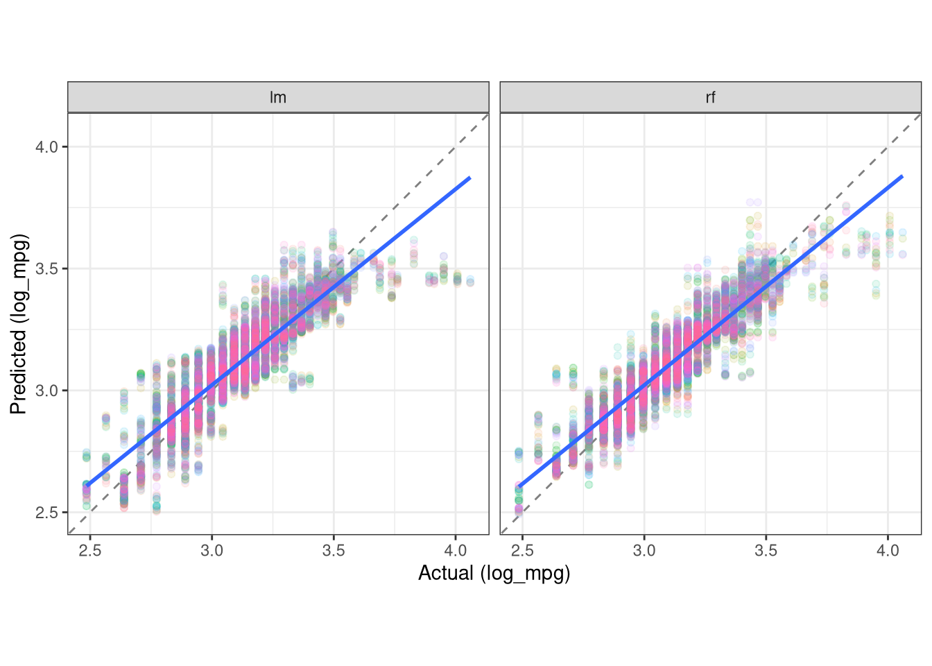

Tune the Random Forest model

# Build a random forest model specification
rf_spec <- rand_forest(mtry = tune(),
                       min_n = tune(),
                       trees = 1000) |> 
    set_engine("ranger", importance = "impurity") |> 
    set_mode("regression")
rf_spec

Random Forest Model Specification (regression)

Main Arguments:
  mtry = tune()
  trees = 1000
  min_n = tune()

Engine-Specific Arguments:
  importance = impurity

Computational engine: ranger

Cross Validation

set.seed(42)
car_folds <- vfold_cv(car_train, v = 10, repeats = 5)

rf_recipe <- recipe(log_mpg ~.,  data = car_train) 
rf_wkfl <- workflow() |> 
  add_recipe(rf_recipe) |> 
  add_model(rf_spec)
rf_wkfl

══ Workflow ════════════════════════════════════════════════════════════════════
Preprocessor: Recipe
Model: rand_forest()

── Preprocessor ────────────────────────────────────────────────────────────────
0 Recipe Steps

── Model ───────────────────────────────────────────────────────────────────────
Random Forest Model Specification (regression)

Main Arguments:
  mtry = tune()
  trees = 1000
  min_n = tune()

Engine-Specific Arguments:
  importance = impurity

Computational engine: ranger

Tune the model

Tip

The next code chunk will take 20 minutes or so to run. Make sure to cache the chunk so that you can rebuild your document without having the code chunk run each time the document is rendered.

doParallel::registerDoParallel()
set.seed(321)
rf_tune <- tune_grid(rf_wkfl, resample = car_folds, grid = 15)
rf_tune

# Tuning results
# 10-fold cross-validation repeated 5 times 
# A tibble: 50 × 5
   splits           id      id2    .metrics          .notes          
   <list>           <chr>   <chr>  <list>            <list>          
 1 <split [823/92]> Repeat1 Fold01 <tibble [30 × 6]> <tibble [0 × 3]>
 2 <split [823/92]> Repeat1 Fold02 <tibble [30 × 6]> <tibble [0 × 3]>
 3 <split [823/92]> Repeat1 Fold03 <tibble [30 × 6]> <tibble [0 × 3]>
 4 <split [823/92]> Repeat1 Fold04 <tibble [30 × 6]> <tibble [0 × 3]>
 5 <split [823/92]> Repeat1 Fold05 <tibble [30 × 6]> <tibble [0 × 3]>
 6 <split [824/91]> Repeat1 Fold06 <tibble [30 × 6]> <tibble [0 × 3]>
 7 <split [824/91]> Repeat1 Fold07 <tibble [30 × 6]> <tibble [0 × 3]>
 8 <split [824/91]> Repeat1 Fold08 <tibble [30 × 6]> <tibble [0 × 3]>
 9 <split [824/91]> Repeat1 Fold09 <tibble [30 × 6]> <tibble [0 × 3]>
10 <split [824/91]> Repeat1 Fold10 <tibble [30 × 6]> <tibble [0 × 3]>
# ℹ 40 more rows

show_best(rf_tune, metric = "rmse")

# A tibble: 5 × 8
   mtry min_n .metric .estimator   mean     n std_err .config              
  <int> <int> <chr>   <chr>       <dbl> <int>   <dbl> <chr>                
1     6     4 rmse    standard   0.0802    50 0.00137 Preprocessor1_Model09
2    10     7 rmse    standard   0.0818    50 0.00138 Preprocessor1_Model13
3     3     2 rmse    standard   0.0836    50 0.00134 Preprocessor1_Model05
4     7    15 rmse    standard   0.0857    50 0.00137 Preprocessor1_Model10
5     3    12 rmse    standard   0.0875    50 0.00134 Preprocessor1_Model06

# rf_param <- tibble(mtry = 6, min_n = 2)
rf_param <- select_best(rf_tune, metric = "rmse")
rf_param

# A tibble: 1 × 3
   mtry min_n .config              
  <int> <int> <chr>                
1     6     4 Preprocessor1_Model09

final_rf_wkfl <- rf_wkfl |> 
  finalize_workflow(rf_param)
final_rf_wkfl

══ Workflow ════════════════════════════════════════════════════════════════════
Preprocessor: Recipe
Model: rand_forest()

── Preprocessor ────────────────────────────────────────────────────────────────
0 Recipe Steps

── Model ───────────────────────────────────────────────────────────────────────
Random Forest Model Specification (regression)

Main Arguments:
  mtry = 6
  trees = 1000
  min_n = 4

Engine-Specific Arguments:
  importance = impurity

Computational engine: ranger

final_rf_fit <- final_rf_wkfl |> 
  fit(car_train)
# Variable importance plot
vip::vip(final_rf_fit) + 
  theme_bw()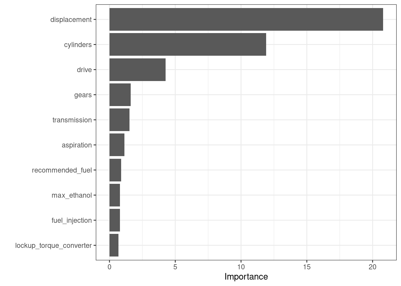

augment(final_rf_fit, new_data = car_test) |> 
  metrics(truth = log_mpg, estimate = .pred) -> RF
RF |> 
  knitr::kable()

.metric	.estimator	.estimate
rmse	standard	0.0788800
rsq	standard	0.8705285
mae	standard	0.0563864

# R-squared plot
augment(final_rf_fit, new_data = car_test) |> 
  ggplot(aes(x = log_mpg, y = .pred)) + 
  geom_point() +
  geom_smooth(method = "gam") +
  geom_abline(lty = "dashed") +
  coord_obs_pred() + 
  theme_bw() + 
  labs(x = "Observed log_mpg",
       y = "Predicted log_mpg",
       title = "R-squared Plot")

library(probably)
augment(final_rf_fit, new_data = car_test) |>
cal_plot_regression(truth = log_mpg, estimate = .pred) + 
  theme_bw()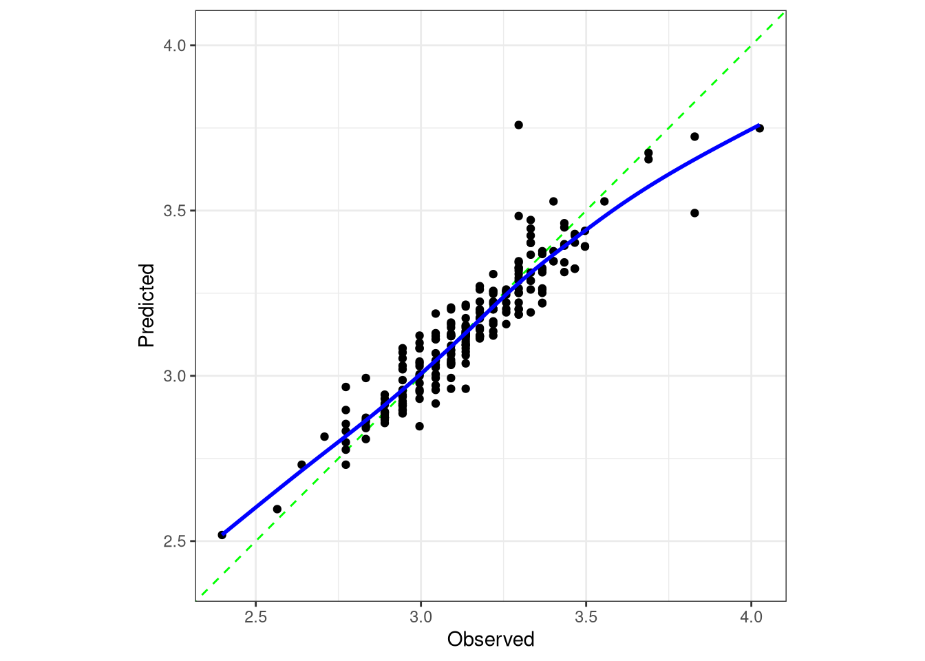

Using Boosting

xgboost_spec <- 
  boost_tree(trees = tune(), min_n = tune(), tree_depth = tune(), 
             learn_rate = tune(), loss_reduction = tune(), 
             sample_size = tune()) |>  
  set_mode("regression") |>  
  set_engine("xgboost") 
xgboost_spec

Boosted Tree Model Specification (regression)

Main Arguments:
  trees = tune()
  min_n = tune()
  tree_depth = tune()
  learn_rate = tune()
  loss_reduction = tune()
  sample_size = tune()

Computational engine: xgboost

xgboost_recipe <- 
  recipe(formula = log_mpg ~  . , data = car_train) |> 
  step_dummy(all_nominal_predictors(), one_hot = TRUE) |> 
  step_zv(all_predictors())  |> 
  step_normalize(all_numeric_predictors()) |> 
  step_corr(all_numeric_predictors(), threshold = 0.9)

xgboost_workflow <- 
  workflow() |>  
  add_recipe(xgboost_recipe) |>  
  add_model(xgboost_spec) 
xgboost_workflow

══ Workflow ════════════════════════════════════════════════════════════════════
Preprocessor: Recipe
Model: boost_tree()

── Preprocessor ────────────────────────────────────────────────────────────────
4 Recipe Steps

• step_dummy()
• step_zv()
• step_normalize()
• step_corr()

── Model ───────────────────────────────────────────────────────────────────────
Boosted Tree Model Specification (regression)

Main Arguments:
  trees = tune()
  min_n = tune()
  tree_depth = tune()
  learn_rate = tune()
  loss_reduction = tune()
  sample_size = tune()

Computational engine: xgboost

Tip

Use cache: true as the next chunk takes a hot minute.

library(finetune) 
# used for tune_race_anova() which...
# after an initial number of resamples have been evaluated, 
# the process eliminates tuning parameter combinations that 
# are unlikely to be the best results using a repeated 
# measure ANOVA model.
set.seed(49)
xgboost_tune <-
  tune_race_anova(xgboost_workflow, resamples = car_folds, grid = 15)
xgboost_tune

# Tuning results
# 10-fold cross-validation repeated 5 times 
# A tibble: 50 × 6
   splits           id      id2    .order .metrics           .notes          
   <list>           <chr>   <chr>   <int> <list>             <list>          
 1 <split [823/92]> Repeat1 Fold03      3 <tibble [30 × 10]> <tibble [1 × 3]>
 2 <split [823/92]> Repeat1 Fold05      1 <tibble [30 × 10]> <tibble [2 × 3]>
 3 <split [824/91]> Repeat1 Fold08      2 <tibble [30 × 10]> <tibble [1 × 3]>
 4 <split [824/91]> Repeat1 Fold07      4 <tibble [12 × 10]> <tibble [0 × 3]>
 5 <split [824/91]> Repeat1 Fold06      5 <tibble [6 × 10]>  <tibble [0 × 3]>
 6 <split [823/92]> Repeat1 Fold01      6 <tibble [4 × 10]>  <tibble [0 × 3]>
 7 <split [823/92]> Repeat1 Fold02      7 <tibble [4 × 10]>  <tibble [0 × 3]>
 8 <split [824/91]> Repeat1 Fold09      8 <tibble [4 × 10]>  <tibble [0 × 3]>
 9 <split [823/92]> Repeat1 Fold04      9 <tibble [4 × 10]>  <tibble [0 × 3]>
10 <split [824/91]> Repeat1 Fold10     10 <tibble [4 × 10]>  <tibble [0 × 3]>
# ℹ 40 more rows

There were issues with some computations:

  - Warning(s) x4: A correlation computation is required, but `estimate` is constant...

Run `show_notes(.Last.tune.result)` for more information.

show_best(xgboost_tune, metric = "rmse")

# A tibble: 5 × 12
  trees min_n tree_depth learn_rate loss_reduction sample_size .metric
  <int> <int>      <int>      <dbl>          <dbl>       <dbl> <chr>  
1  1857    31          2     0.0921   0.0164             0.679 rmse   
2  1571    40         13     0.0611   0.000373           0.421 rmse   
3  1714     7         14     0.0405   0.0000000291       0.743 rmse   
4   429    21          4     0.139    0.0000000001       0.614 rmse   
5   572    15         12     0.210    0.109              0.936 rmse   
# ℹ 5 more variables: .estimator <chr>, mean <dbl>, n <int>, std_err <dbl>,
#   .config <chr>

# xgboost_param <- tibble(trees = 2000, 
#                        min_n = 9, 
#                        tree_depth = 6, 
#                        learn_rate = 0.00681,
#                        loss_reduction = 0.0000000155, 
#                        sample_size = 0.771)
xgboost_param <- select_best(xgboost_tune)
final_xgboost_wkfl <- xgboost_workflow |> 
  finalize_workflow(xgboost_param)
final_xgboost_wkfl

══ Workflow ════════════════════════════════════════════════════════════════════
Preprocessor: Recipe
Model: boost_tree()

── Preprocessor ────────────────────────────────────────────────────────────────
4 Recipe Steps

• step_dummy()
• step_zv()
• step_normalize()
• step_corr()

── Model ───────────────────────────────────────────────────────────────────────
Boosted Tree Model Specification (regression)

Main Arguments:
  trees = 1857
  min_n = 31
  tree_depth = 2
  learn_rate = 0.0921055317689482
  loss_reduction = 0.0163789370695406
  sample_size = 0.678571428571429

Computational engine: xgboost

final_xgboost_fit <- final_xgboost_wkfl |> 
  fit(car_train)

augment(final_xgboost_fit, new_data = car_test) |> 
  metrics(truth = log_mpg, estimate = .pred) -> R5
R5 |> 
  knitr::kable()

.metric	.estimator	.estimate
rmse	standard	0.0940729
rsq	standard	0.8154165
mae	standard	0.0708401

Elastic net

enet_spec <- linear_reg(penalty = tune()) |> 
  set_engine("glmnet") |> 
  set_mode("regression")
enet_spec

Linear Regression Model Specification (regression)

Main Arguments:
  penalty = tune()

Computational engine: glmnet

enet_recipe <- 
  recipe(formula = log_mpg ~  . , data = car_train) |> 
  step_dummy(all_nominal_predictors(), one_hot = TRUE) |> 
  step_zv(all_predictors())  |> 
  step_normalize(all_numeric_predictors()) |> 
  step_corr(all_numeric_predictors(), threshold = 0.9)

enet_workflow <- 
  workflow() |>  
  add_recipe(enet_recipe) |>  
  add_model(enet_spec) 
enet_workflow

══ Workflow ════════════════════════════════════════════════════════════════════
Preprocessor: Recipe
Model: linear_reg()

── Preprocessor ────────────────────────────────────────────────────────────────
4 Recipe Steps

• step_dummy()
• step_zv()
• step_normalize()
• step_corr()

── Model ───────────────────────────────────────────────────────────────────────
Linear Regression Model Specification (regression)

Main Arguments:
  penalty = tune()

Computational engine: glmnet

library(finetune)
set.seed(49)
enet_tune <-
  tune_race_anova(enet_workflow, resamples = car_folds, grid = 15)
enet_tune

# Tuning results
# 10-fold cross-validation repeated 5 times 
# A tibble: 50 × 6
   splits           id      id2    .order .metrics          .notes          
   <list>           <chr>   <chr>   <int> <list>            <list>          
 1 <split [823/92]> Repeat1 Fold03      3 <tibble [30 × 5]> <tibble [1 × 3]>
 2 <split [823/92]> Repeat1 Fold05      1 <tibble [30 × 5]> <tibble [1 × 3]>
 3 <split [824/91]> Repeat1 Fold08      2 <tibble [30 × 5]> <tibble [1 × 3]>
 4 <split [824/91]> Repeat1 Fold07      4 <tibble [24 × 5]> <tibble [0 × 3]>
 5 <split [824/91]> Repeat1 Fold06      5 <tibble [22 × 5]> <tibble [0 × 3]>
 6 <split [823/92]> Repeat1 Fold01      6 <tibble [22 × 5]> <tibble [0 × 3]>
 7 <split [823/92]> Repeat1 Fold02      7 <tibble [22 × 5]> <tibble [0 × 3]>
 8 <split [824/91]> Repeat1 Fold09      8 <tibble [22 × 5]> <tibble [0 × 3]>
 9 <split [823/92]> Repeat1 Fold04      9 <tibble [22 × 5]> <tibble [0 × 3]>
10 <split [824/91]> Repeat1 Fold10     10 <tibble [22 × 5]> <tibble [0 × 3]>
# ℹ 40 more rows

There were issues with some computations:

  - Warning(s) x3: A correlation computation is required, but `estimate` is constant...

Run `show_notes(.Last.tune.result)` for more information.

show_best(enet_tune, metric = "rmse")

# A tibble: 1 × 7
   penalty .metric .estimator  mean     n std_err .config              
     <dbl> <chr>   <chr>      <dbl> <int>   <dbl> <chr>                
1 0.000996 rmse    standard   0.115    50 0.00171 Preprocessor1_Model11

enet_param <- select_best(enet_tune, metric = "rmse")
final_enet_wkfl <- enet_workflow |> 
  finalize_workflow(enet_param)
final_enet_wkfl

══ Workflow ════════════════════════════════════════════════════════════════════
Preprocessor: Recipe
Model: linear_reg()

── Preprocessor ────────────────────────────────────────────────────────────────
4 Recipe Steps

• step_dummy()
• step_zv()
• step_normalize()
• step_corr()

── Model ───────────────────────────────────────────────────────────────────────
Linear Regression Model Specification (regression)

Main Arguments:
  penalty = 0.000996222685531374

Computational engine: glmnet

final_enet_fit <- final_enet_wkfl |> 
  fit(car_train)

augment(final_enet_fit, new_data = car_test) |> 
  metrics(truth = log_mpg, estimate = .pred) -> R6
R6 |> 
  knitr::kable()

.metric	.estimator	.estimate
rmse	standard	0.1064473
rsq	standard	0.7633985
mae	standard	0.0809508

# Print the model object
broom::tidy(final_enet_fit) |> 
  knitr::kable()

term	estimate	penalty
(Intercept)	3.1121513	0.0009962
cylinders	-0.1444559	0.0009962
gears	0.0084966	0.0009962
max_ethanol	-0.0042378	0.0009962
intake_valves_per_cyl	0.0000000	0.0009962
transmission_Automatic	0.0000000	0.0009962
transmission_CVT	0.0481164	0.0009962
transmission_Manual	0.0000000	0.0009962
aspiration_Turbocharged.Supercharged	-0.0103688	0.0009962
lockup_torque_converter_Y	-0.0257989	0.0009962
drive_X2.Wheel.Drive..Front	0.0539045	0.0009962
drive_X2.Wheel.Drive..Rear	0.0000000	0.0009962
drive_X4.Wheel.Drive	-0.0145382	0.0009962
drive_All.Wheel.Drive	-0.0034592	0.0009962
recommended_fuel_Premium.Unleaded.Recommended	0.0137782	0.0009962
recommended_fuel_Premium.Unleaded.Required	0.0000000	0.0009962
recommended_fuel_Regular.Unleaded.Recommended	-0.0008115	0.0009962
fuel_injection_Multipoint.sequential.ignition	-0.0142389	0.0009962

Natural Splines and Interactions

lm_spec <- linear_reg() |> 
  set_engine("lm")
ns_recipe <- recipe(log_mpg ~ ., data = car_train) |> 
  step_ns(displacement, cylinders, gears, deg_free = 6) |> 
  step_interact(~drive:transmission + drive:recommended_fuel)
ns_wkfl <- workflow() |> 
  add_recipe(ns_recipe) |> 
  add_model(lm_spec)
ns_wkfl

══ Workflow ════════════════════════════════════════════════════════════════════
Preprocessor: Recipe
Model: linear_reg()

── Preprocessor ────────────────────────────────────────────────────────────────
2 Recipe Steps

• step_ns()
• step_interact()

── Model ───────────────────────────────────────────────────────────────────────
Linear Regression Model Specification (regression)

Computational engine: lm

final_lm_fit <- ns_wkfl |> 
  fit(car_train)

augment(final_lm_fit, new_data = car_test) |> 
  metrics(truth = log_mpg, estimate = .pred) -> R7
R7 |> 
  knitr::kable()

.metric	.estimator	.estimate
rmse	standard	0.0935618
rsq	standard	0.8197666
mae	standard	0.0694639

broom::tidy(final_lm_fit) |> 
  knitr::kable()

term	estimate	std.error	statistic	p.value
(Intercept)	3.8199245	0.0685005	55.7649217	0.0000000
transmissionCVT	0.1112348	0.0252321	4.4084556	0.0000117
transmissionManual	0.0117752	0.0210889	0.5583622	0.5767406
aspirationTurbocharged/Supercharged	-0.1082848	0.0105613	-10.2530173	0.0000000
lockup_torque_converterY	-0.0812153	0.0162432	-4.9999736	0.0000007
drive2-Wheel Drive, Rear	0.0267326	0.0231243	1.1560408	0.2479815
drive4-Wheel Drive	-0.0946227	0.0693818	-1.3637968	0.1729839
driveAll Wheel Drive	-0.0254093	0.0217824	-1.1665048	0.2437297
max_ethanol	-0.0000903	0.0002151	-0.4200232	0.6745721
recommended_fuelPremium Unleaded Required	-0.0124601	0.0398575	-0.3126149	0.7546481
recommended_fuelRegular Unleaded Recommended	0.0255288	0.0186546	1.3685029	0.1715076
intake_valves_per_cyl	-0.0284054	0.0669422	-0.4243274	0.6714318
exhaust_valves_per_cyl	-0.0635069	0.0615174	-1.0323408	0.3021991
fuel_injectionMultipoint/sequential ignition	-0.0373248	0.0093153	-4.0068477	0.0000668
displacement_ns_1	-0.3615843	0.0382241	-9.4595932	0.0000000
displacement_ns_2	-0.3176055	0.0807107	-3.9351092	0.0000898
displacement_ns_3	-0.4964326	0.0698705	-7.1050404	0.0000000
displacement_ns_4	-0.4479254	0.0704548	-6.3576228	0.0000000
displacement_ns_5	-0.8097319	0.1304069	-6.2092716	0.0000000
displacement_ns_6	-0.7109073	0.0634985	-11.1956491	0.0000000
cylinders_ns_1	0.0750792	0.2045495	0.3670465	0.7136735
cylinders_ns_2	-0.0671265	0.1109896	-0.6048003	0.5454692
cylinders_ns_3	0.0534042	0.1138544	0.4690565	0.6391467
cylinders_ns_4	-0.1620988	0.0994543	-1.6298820	0.1034880
cylinders_ns_5	-0.1105315	0.1406690	-0.7857557	0.4322243
cylinders_ns_6	-0.1231298	0.0845613	-1.4561009	0.1457251
gears_ns_1	-0.0102324	0.0275649	-0.3712124	0.7105696
gears_ns_2	0.0262952	0.0307764	0.8543943	0.3931215
gears_ns_3	0.0281461	0.0318665	0.8832496	0.3773451
gears_ns_4	0.0919127	0.0349123	2.6326768	0.0086215
gears_ns_5	-0.1105689	0.0693967	-1.5932863	0.1114588
gears_ns_6	0.0851329	0.0297666	2.8600177	0.0043374
`drive2-Wheel Drive, Rear_x_transmissionCVT`	0.1027385	0.0734966	1.3978663	0.1625091
`drive4-Wheel Drive_x_transmissionCVT`	0.0068924	0.0481294	0.1432057	0.8861609
`driveAll Wheel Drive_x_transmissionCVT`	-0.0130268	0.0305162	-0.4268796	0.6695725
`drive2-Wheel Drive, Rear_x_transmissionManual`	-0.1129130	0.0210164	-5.3726089	0.0000001
`drive4-Wheel Drive_x_transmissionManual`	-0.0023616	0.0289555	-0.0815580	0.9350170
`driveAll Wheel Drive_x_transmissionManual`	-0.0263497	0.0220420	-1.1954326	0.2322434
`drive2-Wheel Drive, Rear_x_recommended_fuelPremium Unleaded Required`	-0.0077960	0.0428548	-0.1819162	0.8556908
`drive4-Wheel Drive_x_recommended_fuelPremium Unleaded Required`	0.0450673	0.0787188	0.5725098	0.5671244
`driveAll Wheel Drive_x_recommended_fuelPremium Unleaded Required`	-0.0235163	0.0429153	-0.5479706	0.5838525
`drive2-Wheel Drive, Rear_x_recommended_fuelRegular Unleaded Recommended`	-0.1008941	0.0254154	-3.9698099	0.0000779
`drive4-Wheel Drive_x_recommended_fuelRegular Unleaded Recommended`	-0.0417965	0.0704613	-0.5931843	0.5532118
`driveAll Wheel Drive_x_recommended_fuelRegular Unleaded Recommended`	-0.0620341	0.0230943	-2.6861265	0.0073662

Other Formats

Visualize the fuel efficiency distribution

Build a simple linear model

Instructions

Getting started with tidymodels

Training and testing data

Instructions

Train models with tidymodels

Instructions

Evaluate model performance

Instructions

Use the testing data

Bootstrap resampling

Instructions

Plot modeling results

Tune the Random Forest model

Cross Validation

Tune the model

Using Boosting

Elastic net

Natural Splines and Interactions

Getting started with `tidymodels`

Train models with `tidymodels`