A Review of R Modeling Fundamentals

Author

STT 3860

library(tidyverse)

── Attaching core tidyverse packages ──────────────────────── tidyverse 2.0.0 ──
✔ dplyr     1.1.4     ✔ readr     2.1.5
✔ forcats   1.0.0     ✔ stringr   1.5.1
✔ ggplot2   3.5.1     ✔ tibble    3.2.1
✔ lubridate 1.9.4     ✔ tidyr     1.3.1
✔ purrr     1.0.2     
── Conflicts ────────────────────────────────────────── tidyverse_conflicts() ──
✖ dplyr::filter() masks stats::filter()
✖ dplyr::lag()    masks stats::lag()
ℹ Use the conflicted package (<http://conflicted.r-lib.org/>) to force all conflicts to become errors

library(tidymodels)

── Attaching packages ────────────────────────────────────── tidymodels 1.2.0 ──
✔ broom        1.0.7     ✔ rsample      1.2.1
✔ dials        1.3.0     ✔ tune         1.2.1
✔ infer        1.0.7     ✔ workflows    1.1.4
✔ modeldata    1.4.0     ✔ workflowsets 1.1.0
✔ parsnip      1.2.1     ✔ yardstick    1.3.2
✔ recipes      1.1.0     
── Conflicts ───────────────────────────────────────── tidymodels_conflicts() ──
✖ scales::discard() masks purrr::discard()
✖ dplyr::filter()   masks stats::filter()
✖ recipes::fixed()  masks stringr::fixed()
✖ dplyr::lag()      masks stats::lag()
✖ yardstick::spec() masks readr::spec()
✖ recipes::step()   masks stats::step()
• Dig deeper into tidy modeling with R at https://www.tmwr.org

tidymodels_prefer()

An Example

library(modeldata) # Used for the data crickets
names(crickets)

[1] "species" "temp"    "rate"

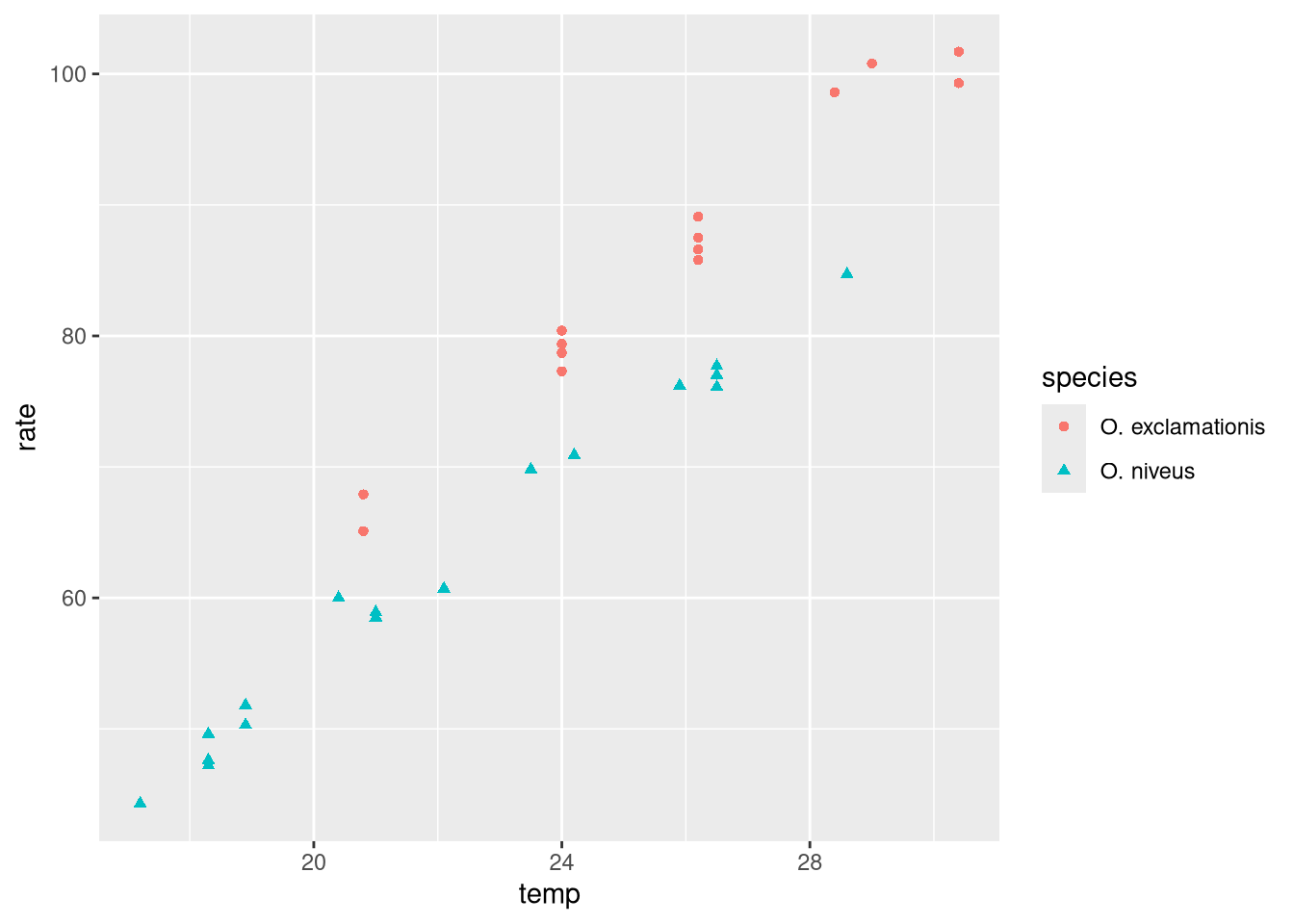
Plot the chirp rate on the y-axis and the temperature on the x-axis, colored by species.

ggplot(data = crickets, 
       aes(x = temp, 
           y = rate, 
           color = species)) + 
  geom_point()

ggplot(data = crickets, 
       aes(x = temp, 
           y = rate, 
           color = species,
           pch = species)) + 
  geom_point()

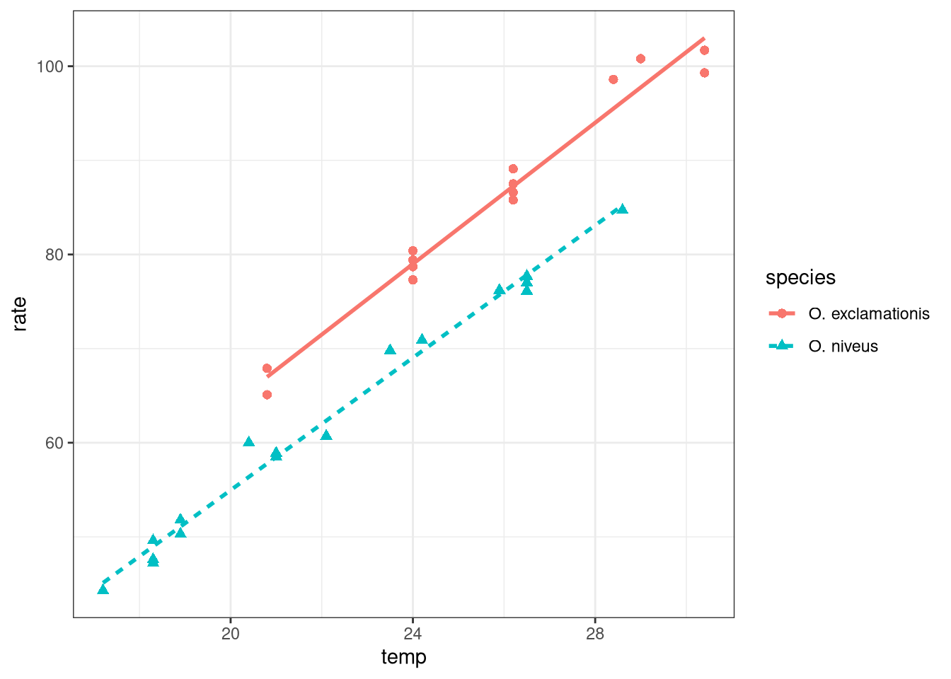
ggplot(data = crickets, 
       aes(x = temp, 
           y = rate, 
           color = species,
           pch = species,
           lty = species)) + 
  geom_point(size = 2) + 
  geom_smooth(method = "lm", se = FALSE, alpha = 0.5) + 
  theme_bw()

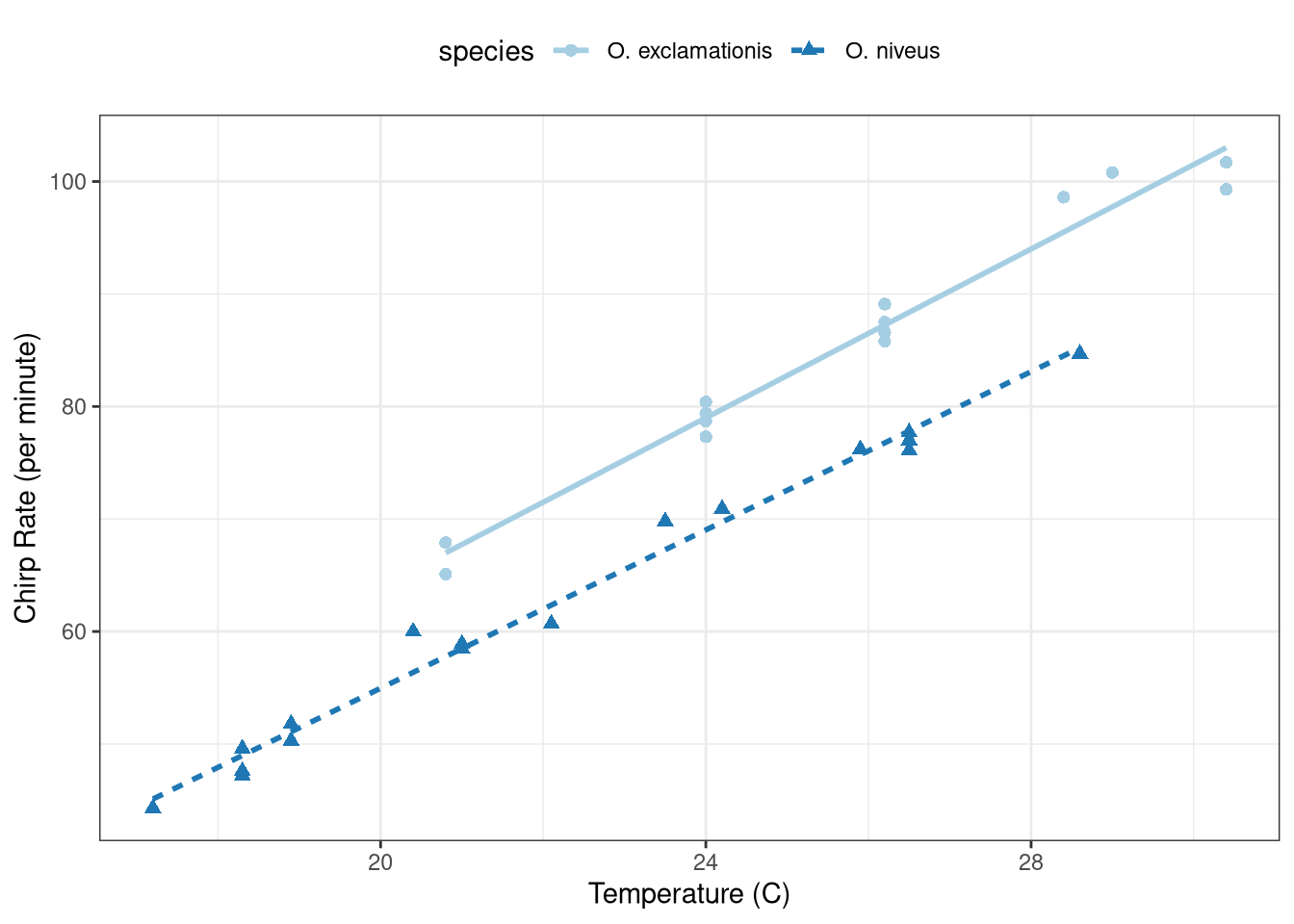
ggplot(data = crickets, 
       aes(x = temp, 
           y = rate, 
           color = species,
           pch = species,
           lty = species)) + 
  geom_point(size = 2) + 
  geom_smooth(method = "lm", se = FALSE, alpha = 0.5) + 
  scale_color_brewer(palette = "Paired") + 
  theme_bw() + 
  labs(x = "Temperature (C)", y = "Chirp Rate (per minute)") + 
  theme(legend.position = "top")

The variable species is stored in R as a factor. Most models need to encode the species data in a numeric format. The model formula rate ~ temp + species, will automatically encode the species column by adding a new numeric column that has a 0 when the species is O. exclamationis and a 1 when the species is O. niveus.

mod_lm <- lm(rate ~ temp + species, data = crickets)
model.matrix(mod_lm) |> 
  bind_cols(SPECIES = crickets$species)

# A tibble: 31 × 4
   `(Intercept)`  temp `speciesO. niveus` SPECIES         
           <dbl> <dbl>              <dbl> <fct>           
 1             1  20.8                  0 O. exclamationis
 2             1  20.8                  0 O. exclamationis
 3             1  24                    0 O. exclamationis
 4             1  24                    0 O. exclamationis
 5             1  24                    0 O. exclamationis
 6             1  24                    0 O. exclamationis
 7             1  26.2                  0 O. exclamationis
 8             1  26.2                  0 O. exclamationis
 9             1  26.2                  0 O. exclamationis
10             1  26.2                  0 O. exclamationis
# ℹ 21 more rows

Tip

There are four levels to the variable heating. The model formula automatically adds three additional binary columns that are binary indicators for three of the heating types. The reference level of the factor (i.e., the first level) is omitted.

library(PASWR2) # For VIT2005
# heating has four levels
mod_example <- lm(totalprice ~ area + heating, data = VIT2005)
model.matrix(mod_example) |> 
  bind_cols(HEATING = VIT2005$heating)

# A tibble: 218 × 6
   `(Intercept)`  area heating3A heating3B heating4A HEATING
           <dbl> <dbl>     <dbl>     <dbl>     <dbl> <fct>  
 1             1  75.3         1         0         0 3A     
 2             1 101.          0         0         1 4A     
 3             1  88.9         1         0         0 3A     
 4             1  62.6         0         0         0 1A     
 5             1 146.          0         0         1 4A     
 6             1  77.2         1         0         0 3A     
 7             1  77.0         0         0         1 4A     
 8             1  62.9         1         0         0 3A     
 9             1  58.5         1         0         0 3A     
10             1  59.2         1         0         0 3A     
# ℹ 208 more rows

The model formula rate ~ temp + species creates a model with different y-intercepts for each species and the same slope.

mod_lm


Call:
lm(formula = rate ~ temp + species, data = crickets)

Coefficients:
     (Intercept)              temp  speciesO. niveus  
          -7.211             3.603           -10.065

# The following may be easier to understand
mod_lm2 <- lm(rate ~ temp + species + 0, data = crickets)
mod_lm2


Call:
lm(formula = rate ~ temp + species + 0, data = crickets)

Coefficients:
                   temp  speciesO. exclamationis         speciesO. niveus  
                  3.603                   -7.211                  -17.276

To get different slopes for each species, consider adding an interaction with one of the following:

mod_int1 <- lm(rate ~ temp + species + temp:species, 
               data = crickets)
mod_int1


Call:
lm(formula = rate ~ temp + species + temp:species, data = crickets)

Coefficients:
          (Intercept)                   temp       speciesO. niveus  
              -11.041                  3.751                 -4.348  
temp:speciesO. niveus  
               -0.234

mod_int2 <- lm(rate ~ temp*species, 
               data = crickets)
mod_int2


Call:
lm(formula = rate ~ temp * species, data = crickets)

Coefficients:
          (Intercept)                   temp       speciesO. niveus  
              -11.041                  3.751                 -4.348  
temp:speciesO. niveus  
               -0.234

mod_int3 <- lm(rate ~ (temp + species)^2, 
               data = crickets)
mod_int3


Call:
lm(formula = rate ~ (temp + species)^2, data = crickets)

Coefficients:
          (Intercept)                   temp       speciesO. niveus  
              -11.041                  3.751                 -4.348  
temp:speciesO. niveus  
               -0.234

Write out the two separate lines from mod_int1.

\[\widehat{\text{rate}} = (-11.041) + (3.751)\cdot \text{temp}\]

\[\widehat{\text{rate}} = (-11.041 -4.348) + (3.751 - 0.234)\cdot \text{temp}\]

The output/models may be easier to understand with:

mod_int4 <- lm(rate ~ (temp + species + temp:species) + 0, 
               data = crickets)
mod_int4


Call:
lm(formula = rate ~ (temp + species + temp:species) + 0, data = crickets)

Coefficients:
                   temp  speciesO. exclamationis         speciesO. niveus  
                  3.751                  -11.041                  -15.389  
  temp:speciesO. niveus  
                 -0.234

Is the interaction term warranted?

mod_reduced <- lm(rate ~ temp + species,
                  data = crickets)
mod_full <- lm(rate ~ temp + species + temp:species,
               data = crickets)
anova(mod_reduced, mod_full) |> 
  tidy() -> ans
ans |> 
  knitr::kable()

term	df.residual	rss	df	sumsq	statistic	p.value
rate ~ temp + species	28	89.34987	NA	NA	NA	NA
rate ~ temp + species + temp:species	27	85.07409	1	4.275779	1.357006	0.2542464

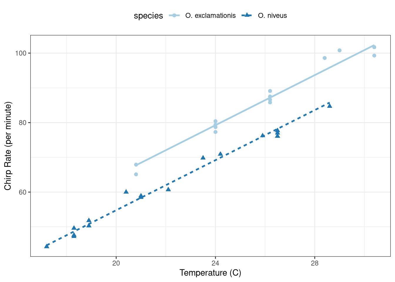
The p-value of 0.25 suggests \(\beta_3 = 0\). The interaction term is not warranted and should be dropped from the model.

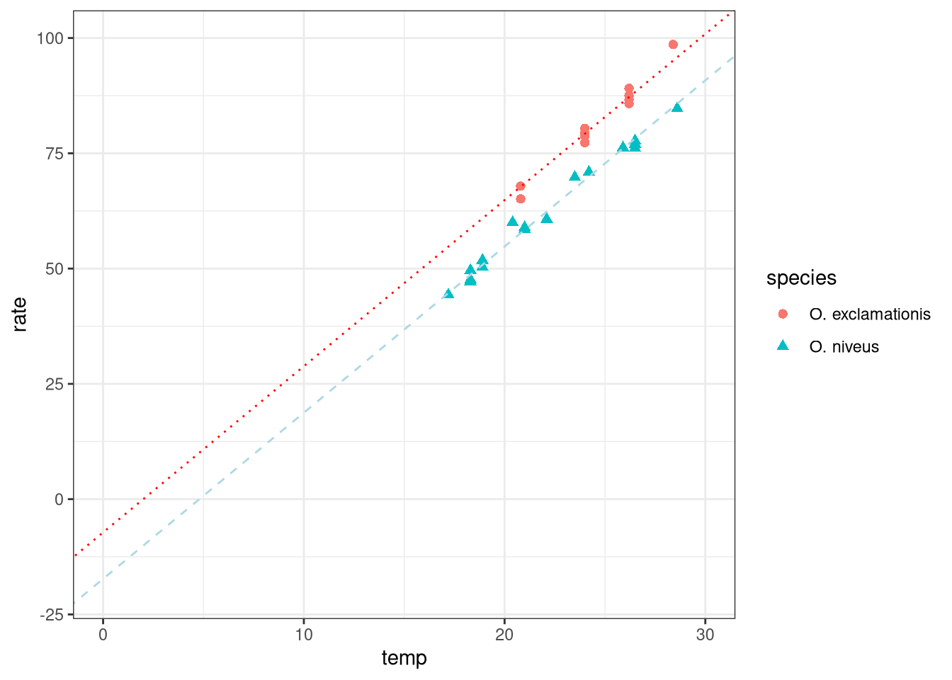
The model is a parallel slopes model and is shown in Figure 1.

ggplot(data = crickets, 
       aes(x = temp, 
           y = rate, 
           color = species,
           pch = species,
           lty = species)) + 
  geom_point(size = 2) + 
  moderndive::geom_parallel_slopes(se = FALSE, alpha = 0.5) + 
  scale_color_brewer(palette = "Paired") + 
  theme_bw() + 
  labs(x = "Temperature (C)", y = "Chirp Rate (per minute)") + 
  theme(legend.position = "top")

Figure 1: Parallel slopes model of chirp rate versus temperature for different species

Or using the coefficients from mod_lm:

mod_lm


Call:
lm(formula = rate ~ temp + species, data = crickets)

Coefficients:
     (Intercept)              temp  speciesO. niveus  
          -7.211             3.603           -10.065

ggplot(data = crickets, 
       aes(x = temp, 
           y = rate, 
           color = species,
           pch = species,
           lty = species)) + 
  geom_point(size = 2) + 
  geom_abline(intercept = -7.211, slope = 3.603, lty = "dotted", color = "red") + 
  geom_abline(intercept = -17.276, slope = 3.603, lty = "dashed", color = "lightblue") + 
  theme_bw() + 
  xlim(0, 30) + 
  ylim(-20, 100)

mtcars |> select(-mpg)

                    cyl  disp  hp drat    wt  qsec vs am gear carb
Mazda RX4             6 160.0 110 3.90 2.620 16.46  0  1    4    4
Mazda RX4 Wag         6 160.0 110 3.90 2.875 17.02  0  1    4    4
Datsun 710            4 108.0  93 3.85 2.320 18.61  1  1    4    1
Hornet 4 Drive        6 258.0 110 3.08 3.215 19.44  1  0    3    1
Hornet Sportabout     8 360.0 175 3.15 3.440 17.02  0  0    3    2
Valiant               6 225.0 105 2.76 3.460 20.22  1  0    3    1
Duster 360            8 360.0 245 3.21 3.570 15.84  0  0    3    4
Merc 240D             4 146.7  62 3.69 3.190 20.00  1  0    4    2
Merc 230              4 140.8  95 3.92 3.150 22.90  1  0    4    2
Merc 280              6 167.6 123 3.92 3.440 18.30  1  0    4    4
Merc 280C             6 167.6 123 3.92 3.440 18.90  1  0    4    4
Merc 450SE            8 275.8 180 3.07 4.070 17.40  0  0    3    3
Merc 450SL            8 275.8 180 3.07 3.730 17.60  0  0    3    3
Merc 450SLC           8 275.8 180 3.07 3.780 18.00  0  0    3    3
Cadillac Fleetwood    8 472.0 205 2.93 5.250 17.98  0  0    3    4
Lincoln Continental   8 460.0 215 3.00 5.424 17.82  0  0    3    4
Chrysler Imperial     8 440.0 230 3.23 5.345 17.42  0  0    3    4
Fiat 128              4  78.7  66 4.08 2.200 19.47  1  1    4    1
Honda Civic           4  75.7  52 4.93 1.615 18.52  1  1    4    2
Toyota Corolla        4  71.1  65 4.22 1.835 19.90  1  1    4    1
Toyota Corona         4 120.1  97 3.70 2.465 20.01  1  0    3    1
Dodge Challenger      8 318.0 150 2.76 3.520 16.87  0  0    3    2
AMC Javelin           8 304.0 150 3.15 3.435 17.30  0  0    3    2
Camaro Z28            8 350.0 245 3.73 3.840 15.41  0  0    3    4
Pontiac Firebird      8 400.0 175 3.08 3.845 17.05  0  0    3    2
Fiat X1-9             4  79.0  66 4.08 1.935 18.90  1  1    4    1
Porsche 914-2         4 120.3  91 4.43 2.140 16.70  0  1    5    2
Lotus Europa          4  95.1 113 3.77 1.513 16.90  1  1    5    2
Ford Pantera L        8 351.0 264 4.22 3.170 14.50  0  1    5    4
Ferrari Dino          6 145.0 175 3.62 2.770 15.50  0  1    5    6
Maserati Bora         8 301.0 335 3.54 3.570 14.60  0  1    5    8
Volvo 142E            4 121.0 109 4.11 2.780 18.60  1  1    4    2

purrr::map(mtcars |> select(-mpg), cor.test, y = mtcars$mpg)

$cyl

    Pearson's product-moment correlation

data:  .x[[i]] and mtcars$mpg
t = -8.9197, df = 30, p-value = 6.113e-10
alternative hypothesis: true correlation is not equal to 0
95 percent confidence interval:
 -0.9257694 -0.7163171
sample estimates:
      cor 
-0.852162 


$disp

    Pearson's product-moment correlation

data:  .x[[i]] and mtcars$mpg
t = -8.7472, df = 30, p-value = 9.38e-10
alternative hypothesis: true correlation is not equal to 0
95 percent confidence interval:
 -0.9233594 -0.7081376
sample estimates:
       cor 
-0.8475514 


$hp

    Pearson's product-moment correlation

data:  .x[[i]] and mtcars$mpg
t = -6.7424, df = 30, p-value = 1.788e-07
alternative hypothesis: true correlation is not equal to 0
95 percent confidence interval:
 -0.8852686 -0.5860994
sample estimates:
       cor 
-0.7761684 


$drat

    Pearson's product-moment correlation

data:  .x[[i]] and mtcars$mpg
t = 5.096, df = 30, p-value = 1.776e-05
alternative hypothesis: true correlation is not equal to 0
95 percent confidence interval:
 0.4360484 0.8322010
sample estimates:
      cor 
0.6811719 


$wt

    Pearson's product-moment correlation

data:  .x[[i]] and mtcars$mpg
t = -9.559, df = 30, p-value = 1.294e-10
alternative hypothesis: true correlation is not equal to 0
95 percent confidence interval:
 -0.9338264 -0.7440872
sample estimates:
       cor 
-0.8676594 


$qsec

    Pearson's product-moment correlation

data:  .x[[i]] and mtcars$mpg
t = 2.5252, df = 30, p-value = 0.01708
alternative hypothesis: true correlation is not equal to 0
95 percent confidence interval:
 0.08195487 0.66961864
sample estimates:
     cor 
0.418684 


$vs

    Pearson's product-moment correlation

data:  .x[[i]] and mtcars$mpg
t = 4.8644, df = 30, p-value = 3.416e-05
alternative hypothesis: true correlation is not equal to 0
95 percent confidence interval:
 0.4103630 0.8223262
sample estimates:
      cor 
0.6640389 


$am

    Pearson's product-moment correlation

data:  .x[[i]] and mtcars$mpg
t = 4.1061, df = 30, p-value = 0.000285
alternative hypothesis: true correlation is not equal to 0
95 percent confidence interval:
 0.3175583 0.7844520
sample estimates:
      cor 
0.5998324 


$gear

    Pearson's product-moment correlation

data:  .x[[i]] and mtcars$mpg
t = 2.9992, df = 30, p-value = 0.005401
alternative hypothesis: true correlation is not equal to 0
95 percent confidence interval:
 0.1580618 0.7100628
sample estimates:
      cor 
0.4802848 


$carb

    Pearson's product-moment correlation

data:  .x[[i]] and mtcars$mpg
t = -3.6157, df = 30, p-value = 0.001084
alternative hypothesis: true correlation is not equal to 0
95 percent confidence interval:
 -0.7546480 -0.2503183
sample estimates:
       cor 
-0.5509251

corr_res <- purrr::map(mtcars |> select(-mpg), cor.test, y = mtcars$mpg)
corr_res[[10]]


    Pearson's product-moment correlation

data:  .x[[i]] and mtcars$mpg
t = -3.6157, df = 30, p-value = 0.001084
alternative hypothesis: true correlation is not equal to 0
95 percent confidence interval:
 -0.7546480 -0.2503183
sample estimates:
       cor 
-0.5509251

corr_res[[10]] |> 
broom::tidy()

# A tibble: 1 × 8
  estimate statistic p.value parameter conf.low conf.high method     alternative
     <dbl>     <dbl>   <dbl>     <int>    <dbl>     <dbl> <chr>      <chr>      
1   -0.551     -3.62 0.00108        30   -0.755    -0.250 Pearson's… two.sided

corr_res |> 
  map_dfr(tidy, .id = "predictor") -> output 
output |> 
  knitr::kable()

predictor	estimate	statistic	p.value	parameter	conf.low	conf.high	method	alternative
cyl	-0.8521620	-8.919699	0.0000000	30	-0.9257694	-0.7163171	Pearson’s product-moment correlation	two.sided
disp	-0.8475514	-8.747151	0.0000000	30	-0.9233594	-0.7081376	Pearson’s product-moment correlation	two.sided
hp	-0.7761684	-6.742388	0.0000002	30	-0.8852686	-0.5860994	Pearson’s product-moment correlation	two.sided
drat	0.6811719	5.096042	0.0000178	30	0.4360484	0.8322010	Pearson’s product-moment correlation	two.sided
wt	-0.8676594	-9.559044	0.0000000	30	-0.9338264	-0.7440872	Pearson’s product-moment correlation	two.sided
qsec	0.4186840	2.525213	0.0170820	30	0.0819549	0.6696186	Pearson’s product-moment correlation	two.sided
vs	0.6640389	4.864385	0.0000342	30	0.4103630	0.8223262	Pearson’s product-moment correlation	two.sided
am	0.5998324	4.106127	0.0002850	30	0.3175583	0.7844520	Pearson’s product-moment correlation	two.sided
gear	0.4802848	2.999191	0.0054009	30	0.1580618	0.7100628	Pearson’s product-moment correlation	two.sided
carb	-0.5509251	-3.615750	0.0010844	30	-0.7546480	-0.2503183	Pearson’s product-moment correlation	two.sided

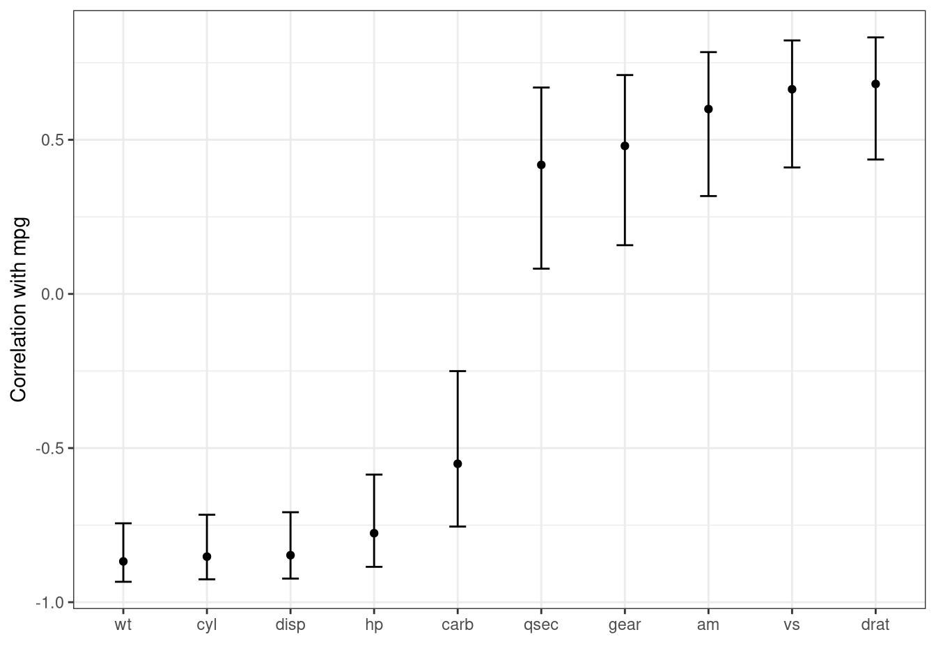
Create a graph with output.

ggplot(data = output, aes(x = fct_reorder(predictor, estimate))) + 
  geom_point(aes(y = estimate)) + 
  geom_errorbar(aes(ymin = conf.low, ymax = conf.high), width = 0.2) + 
  labs(x = "", y = "Correlation with mpg") + 
  theme_bw()

Figure 2: Correlations (and 95% confidence intervals) between predictors and the outcome in the mtcars data set.

Combing Base `R` Models and Tidyverse

crickets |> 
  group_nest(species) |> 
  knitr::kable()

species	data
O. exclamationis	20.8, 20.8, 24.0, 24.0, 24.0, 24.0, 26.2, 26.2, 26.2, 26.2, 28.4, 29.0, 30.4, 30.4, 67.9, 65.1, 77.3, 78.7, 79.4, 80.4, 85.8, 86.6, 87.5, 89.1, 98.6, 100.8, 99.3, 101.7
O. niveus	17.2, 18.3, 18.3, 18.3, 18.9, 18.9, 20.4, 21.0, 21.0, 22.1, 23.5, 24.2, 25.9, 26.5, 26.5, 26.5, 28.6, 44.3, 47.2, 47.6, 49.6, 50.3, 51.8, 60.0, 58.5, 58.9, 60.7, 69.8, 70.9, 76.2, 76.1, 77.0, 77.7, 84.7

crickets |> 
  group_nest(species) |> 
  mutate(model = map(data, ~lm(rate ~ temp, data = .x)))

# A tibble: 2 × 3
  species                        data model 
  <fct>            <list<tibble[,2]>> <list>
1 O. exclamationis           [14 × 2] <lm>  
2 O. niveus                  [17 × 2] <lm>

#
crickets |> 
  group_nest(species) |> 
  mutate(model = map(data, ~lm(rate ~ temp, data = .x))) |> 
  mutate(coef = map(model, tidy))

# A tibble: 2 × 4
  species                        data model  coef            
  <fct>            <list<tibble[,2]>> <list> <list>          
1 O. exclamationis           [14 × 2] <lm>   <tibble [2 × 5]>
2 O. niveus                  [17 × 2] <lm>   <tibble [2 × 5]>

#
crickets |> 
  group_nest(species) |> 
  mutate(model = map(data, ~lm(rate ~ temp, data = .x))) |> 
  mutate(coef = map(model, tidy)) |> 
  select(species, coef) |> 
  unnest(cols = c(coef))

# A tibble: 4 × 6
  species          term        estimate std.error statistic  p.value
  <fct>            <chr>          <dbl>     <dbl>     <dbl>    <dbl>
1 O. exclamationis (Intercept)   -11.0      4.77      -2.32 3.90e- 2
2 O. exclamationis temp            3.75     0.184     20.4  1.10e-10
3 O. niveus        (Intercept)   -15.4      2.35      -6.56 9.07e- 6
4 O. niveus        temp            3.52     0.105     33.6  1.57e-15

An Example

Is the interaction term warranted?

Combing Base R Models and Tidyverse

Combing Base `R` Models and Tidyverse