Multiple logistic regression looking at wines

class: top, right, inverse, title-slide

# Multiple logistic regression looking at wines
### Zach Mullis, Matt Goard, Ben Tibbits, Sebastien Lee
### updated: 2021-03-15

---

class: inverse, center, middle

---
Dr A's comments

Model:

```r
wines2 <- wines %>% 
  mutate(color = ifelse(color == "red", 1, 0))
# str(wines2)
modA <- glm(color ~ sulphates, data = wines2, family = "binomial")
summary(modA)
```

```

Call:
glm(formula = color ~ sulphates, family = "binomial", data = wines2)

Deviance Residuals: 
    Min       1Q   Median       3Q      Max  
-2.7623  -0.6361  -0.4279  -0.2144   2.5790

Coefficients:
            Estimate Std. Error z value Pr(>|z|)    
(Intercept)  -6.4050     0.1684  -38.03   <2e-16 ***
sulphates     9.4425     0.2872   32.88   <2e-16 ***
---
Signif. codes:  0 '***' 0.001 '**' 0.01 '*' 0.05 '.' 0.1 ' ' 1

(Dispersion parameter for binomial family taken to be 1)

Null deviance: 7251.0  on 6496  degrees of freedom
Residual deviance: 5617.5  on 6495  degrees of freedom
AIC: 5621.5

Number of Fisher Scoring iterations: 5
```

---

```r
nullmod <- glm(color ~ 1, family="binomial", data = wines2)
PR2 <- 1 - logLik(modA)/logLik(nullmod)
PR2 # McFadden's R2 --- Can we get a better model?
```

```
'log Lik.' 0.2252801 (df=2)
```

```r
modB <- glm(color ~ density + chlorides, data = wines2, family = "binomial")
# summary(modB)
PR2 <- 1 - logLik(modB)/logLik(nullmod)
PR2 # McFadden's R2 --- Can we get a better model?
```

```
'log Lik.' 0.3733582 (df=3)
```

```r
modC <- glm(color ~ ., data = wines2, family = "binomial")
# summary(modC)
PR2 <- 1 - logLik(modC)/logLik(nullmod)
PR2 # McFadden's R2 --- Can we get a better model?
```

```
'log Lik.' 0.9414927 (df=13)
```

---
How well are we doing?

```r
wines$color <- as.factor(wines$color)
WT <- predict(modC, type ="response")
WT <- (ifelse(WT > .5, "red", "white"))
p_class <- factor(WT, levels = c("red", "white"))
library(caret)
confusionMatrix(p_class, wines$color)
```

```
Confusion Matrix and Statistics

Reference
Prediction  red white
     red   1580    11
     white   19  4887
                                          
               Accuracy : 0.9954          
                 95% CI : (0.9934, 0.9969)
    No Information Rate : 0.7539          
    P-Value [Acc > NIR] : <2e-16          
                                          
                  Kappa : 0.9875          
                                          
 Mcnemar's Test P-Value : 0.2012          
                                          
            Sensitivity : 0.9881          
            Specificity : 0.9978          
         Pos Pred Value : 0.9931          
         Neg Pred Value : 0.9961          
             Prevalence : 0.2461          
         Detection Rate : 0.2432          
   Detection Prevalence : 0.2449          
      Balanced Accuracy : 0.9929          
                                          
       'Positive' Class : red             
                                          
```

---

```r
ggplot(data = wines2, aes(x = sulphates, y = color)) +
  geom_jitter(width = 0, height = 0.05, alpha = 0.1) +
  theme_bw() +
  geom_smooth(method = "glm", se = FALSE, 
              method.args = list(family = binomial(link = "logit")),
              color = "red")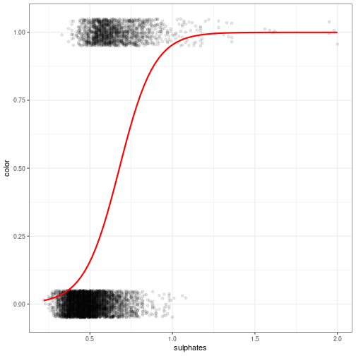
```

![](xariganSlides_files/figure-html/unnamed-chunk-4-1.png)

---

# assumptions of logistic functions:

---
# Here is a plot of the residuals

---
class: inverse, center, middle

# We discovered that...

---

# Using `ggplot2` to illustrate Sulphates, color, and quality together

???
Write everything you want to say about the model here.  Pressing shift p in the slides will put you in presentation mode.

---

# Showing Quality as a relationship of alcohol between red and whites

## In conclusion:

???
if you want to hide notes that you can use later, doing ??? lets you have a hidden section