Tree-Based Methods

Published

Last modified on March 15, 2025 15:38:02 Eastern Daylight Time

Crediting the materials

The descriptions of tree-based methods in this document are taken primarily from An Introduction to Statistical Learning with Applications in R while most of the coding ideas for tidymodels are gleaned from Tidy Modeling with R: A framework for Modeling in the Tidyverse.

Advantages and Disadvantages of Trees

Pros

  • Trees are very easy to explain to people. In fact, they are even easier to explain than linear regression!

  • Some people believe that decision trees more closely mirror human decision-making than do regression and classification approaches.

  • Trees can be displayed graphically, and are easily interpreted even by a non-expert (especially if they are small).

  • Trees can easily handle qualitative predictors without the need to create dummy variables (model.matrix()).

Cons

  • Trees generally do not have the same level of predictive accuracy as some of the other regression and classification approaches.

  • Trees suffer from high variance. This means if we split the training data into two parts at random, and fit a decision tree to both halves, the results that we get could be quite different. In contrast, a procedure with low variance will yield similar results if applied repeatedly to distinct data sets.

How do we improve on a single tree?

By aggregating many decision trees, using methods like bagging, random forests, and boosting, the predictive performance of trees can be substantially improved!

The Basics of Decision Trees

Decision trees can be applied to both regression and classification problems. We first consider regression problems, and then move on to classification problems.

Predicting Baseball Players’ Salaries Using Regression Trees

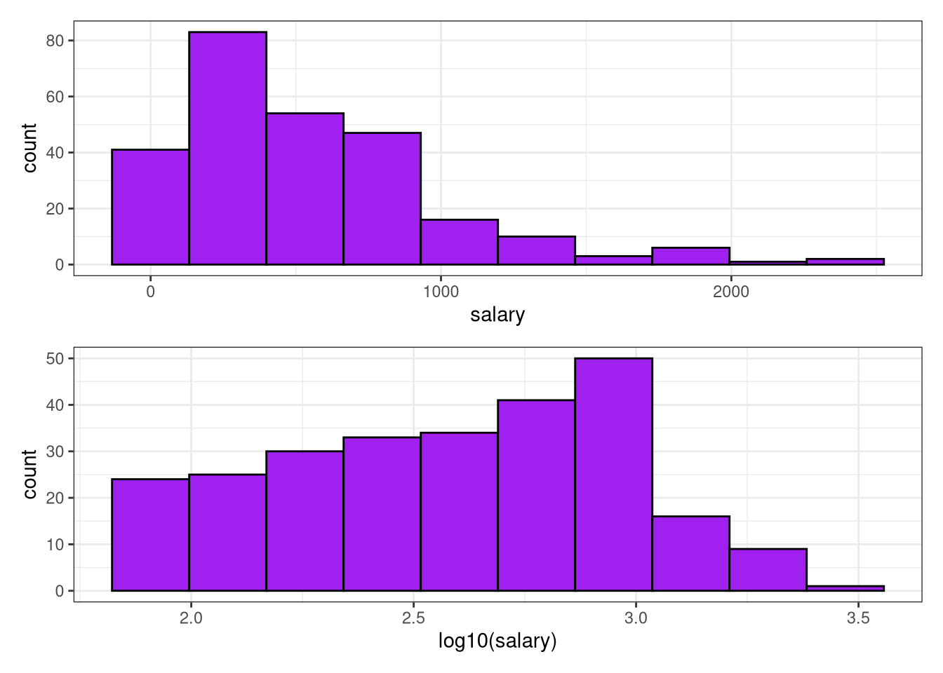
We use the Hitters data set to predict a baseball player’s Salary based on Years (the number of years that he has played in the major leagues) and Hits (the number of hits that he made in the previous year). We first remove observations that are missing Salary values, and log-transform Salary so that its distribution has more of a typical bell-shape. (Recall that Salary is measured in thousands of dollars.)

library(tidymodels)
library(tidyverse)
library(ISLR2)
library(janitor) # standardize variable names
tidymodels_prefer()
Hitters <- na.omit(Hitters) |> 
  clean_names() |> 
  as_tibble()
names(Hitters)
 [1] "at_bat"     "hits"       "hm_run"     "runs"       "rbi"       
 [6] "walks"      "years"      "c_at_bat"   "c_hits"     "c_hm_run"  
[11] "c_runs"     "crbi"       "c_walks"    "league"     "division"  
[16] "put_outs"   "assists"    "errors"     "salary"     "new_league"
ggplot(data = Hitters, aes(x = salary)) + 
  geom_histogram(bins = 10, color = "black", fill = "purple") + 
  theme_bw() -> p1
ggplot(data = Hitters, aes(x = log10(salary))) + 
  geom_histogram(bins = 10, color = "black", fill = "purple") + 
  theme_bw() -> p2
library(patchwork)
p1/p2

# Put salary on log10 scale
Hitters <- Hitters |> 
  mutate(salary = log10(salary))

We start by creating a tree “specification” using the parsnip package which was loaded with the tidymodels bundle.

tree_spec <- decision_tree() |> 
  set_engine("rpart") |> 
  set_mode("regression")
tree_spec
Decision Tree Model Specification (regression)

Computational engine: rpart 

With a model specification and data we are ready to fit a model. The first model we will consider uses both year and hits as predictors.

tree_fit <- tree_spec |> 
  fit(salary ~ years + hits, data = Hitters)

When we look at the model output, we see an informative summary of the model.

tree_fit
parsnip model object

n= 263 

node), split, n, deviance, yval
      * denotes terminal node

 1) root 263 39.0716200 2.574160  
   2) years< 4.5 90  7.9883020 2.217851  
     4) years< 3.5 62  4.3397050 2.124487  
       8) hits< 114 43  3.2338760 2.053078 *
       9) hits>=114 19  0.3903227 2.286097 *
     5) years>=3.5 28  1.9114650 2.424585 *
   3) years>=4.5 173 13.7130700 2.759523  
     6) hits< 117.5 90  5.2988020 2.605063  
      12) years< 6.5 26  1.3651130 2.470669 *
      13) years>=6.5 64  3.2733010 2.659661  
        26) hits< 50.5 12  0.5072597 2.488515 *
        27) hits>=50.5 52  2.3334350 2.699156 *
     7) hits>=117.5 83  3.9387920 2.927009 *

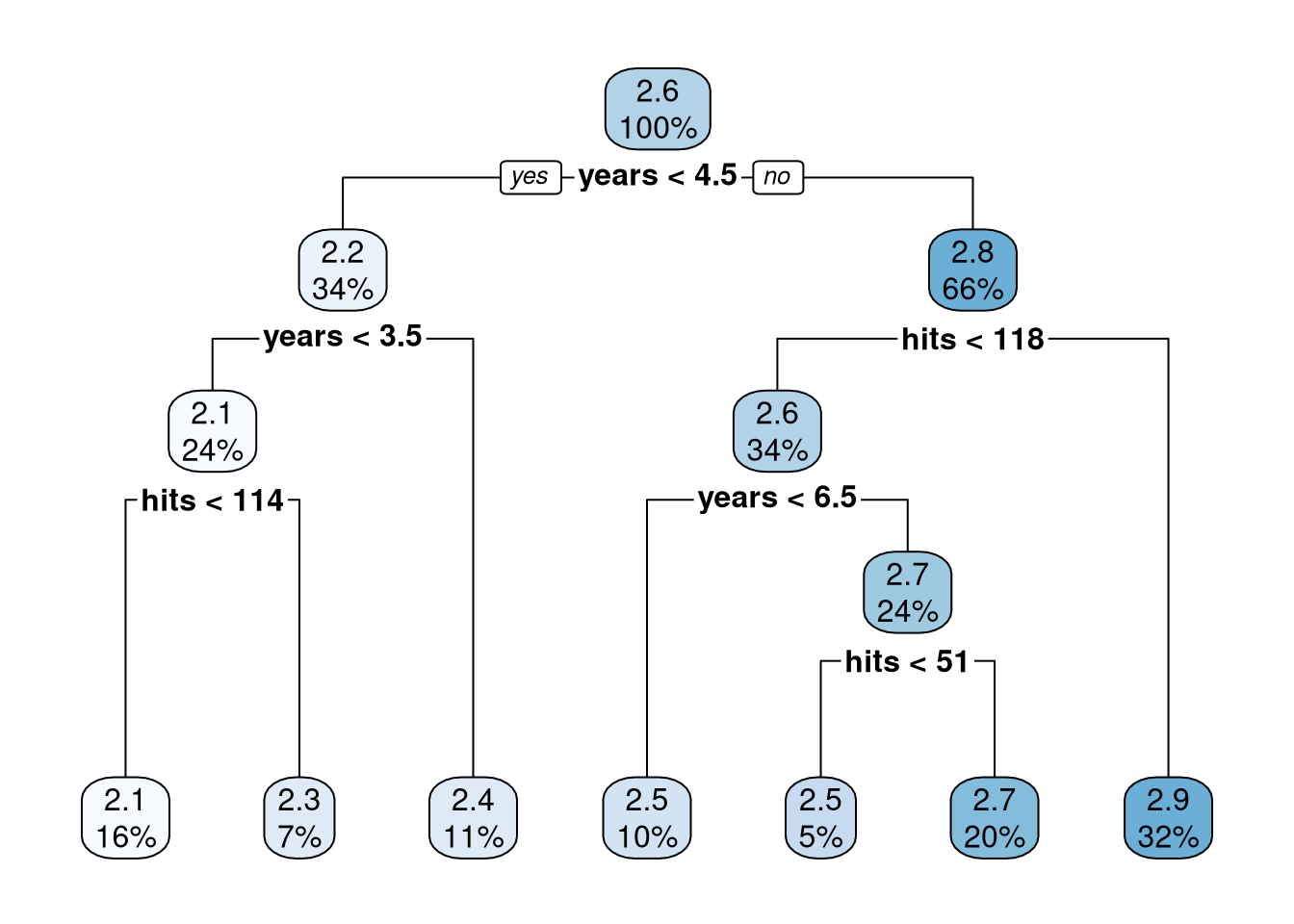
Once the tree gets more than a couple of nodes, it can become hard to read the printed diagram. The rpart.plot package provides functions to let us easily visualize the decision tree. The function rpart.plot only works with rpart trees so we will use the extract_fit_engine() from the parsnip package.

tree_fit |> 
  extract_fit_engine() |> 
  rpart.plot::rpart.plot(roundint = FALSE)

Figure 1: Tree Model for predicting salary based on years and hits
# Print Rules
tree_fit |> 
  extract_fit_engine() |> 
  rpart.plot::rpart.rules(roundint = FALSE)
 salary                                              
    2.1 when years <  3.5        & hits <  114       
    2.3 when years <  3.5        & hits >=        114
    2.4 when years is 3.5 to 4.5                     
    2.5 when years is 4.5 to 6.5 & hits <  118       
    2.5 when years >=        6.5 & hits <   51       
    2.7 when years >=        6.5 & hits is  51 to 118
    2.9 when years >=        4.5 & hits >=        118
Tip

Each node in Figure 1 shows:

  • the predicted value,
  • the percentage of observations in the node.

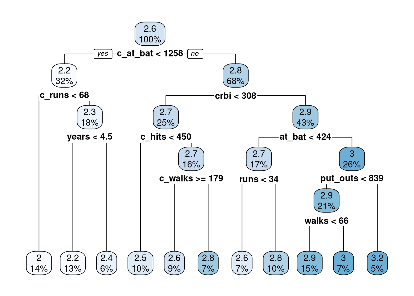
For example, all observations (100%) are in the first node and the top number (2.6) is the average salary (in log10) of all players in Hitters. That is \(10^{2.574160}=375.1112\) and remembering that salary is in thousands of dollars, the average salary for all 263 players is $375,111. Moving to the left for players with fewer than 4.5 years in the league we see that note contains 34% of the players and their predicted salary is \(10^{2.217851}\times 1000\) = $165,140.

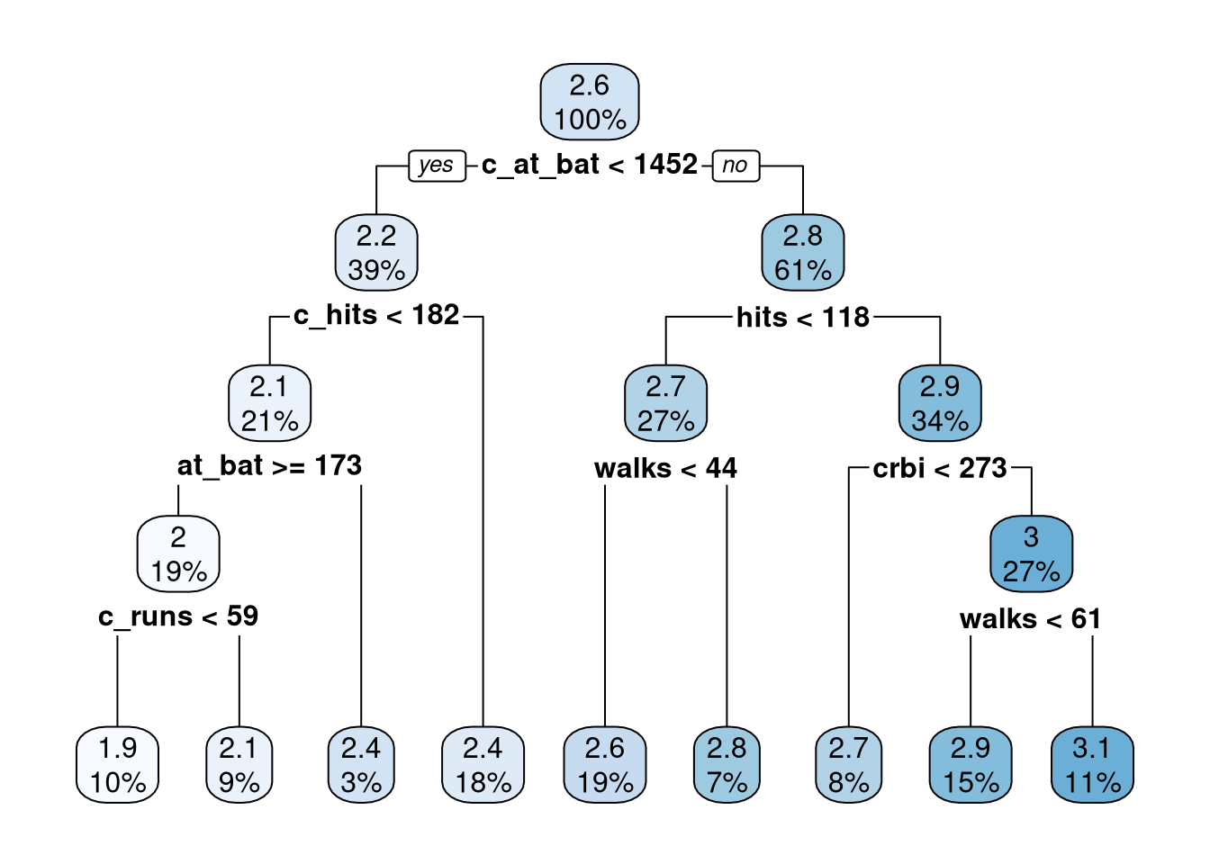
Next we consider a model that uses all of the variables in Hitters.

tree_fit2 <- tree_spec |> 
  fit(salary ~ ., data = Hitters)
tree_fit2 |> 
  extract_fit_engine() |> 
  rpart.plot::rpart.plot(roundint = FALSE)

Figure 2: Tree Model for predicting salary based on all predictors in Hitters

Evaluating the Performance of your Model

To evaluate model performance, we will use the metrics() function from the yardstick package which was loaded with the tidyverse bundle.

augment(tree_fit2, new_data = Hitters) |> 
  metrics(truth = salary, estimate = .pred) -> R1
R1 |> 
  knitr::kable()
.metric .estimator .estimate
rmse standard 0.1823249
rsq standard 0.7762381
mae standard 0.1339507

The mean absolute error (mae) is \(10^{0.1339507}\cdot 1000\) = $1,361.29 and the model’s \(R^2\) value is 77.62% which is not bad. However, this model was fit on the entire data set and the model is likely overfitting the data. Next we refit the model using a training set and tune the model’s complexity parameter (cost_complexity). After tuning the cost_complexity, we evaluate the model’s performance on the test set to get an idea of how the model will perform on data it has not seen.

Splitting the Data

set.seed(314)
hitters_split <- initial_split(Hitters)
hitters_train <- training(hitters_split)
hitters_test <- testing(hitters_split)
dim(hitters_train)
[1] 197  20
dim(hitters_test)
[1] 66 20
hitters_folds <- vfold_cv(hitters_train, v = 10, repeats = 5)
tree_spec <- decision_tree(cost_complexity = tune()) |> 
  set_engine("rpart") |> 
  set_mode("regression")
tree_spec
Decision Tree Model Specification (regression)

Main Arguments:
  cost_complexity = tune()

Computational engine: rpart 
tree_recipe <- recipe(formula = salary ~ ., data = hitters_train) 
tree_wkfl <- workflow() |> 
  add_recipe(tree_recipe) |> 
  add_model(tree_spec) 
set.seed(8675)
tree_tune <-
  tune_grid(tree_wkfl, resamples = hitters_folds, grid = 15)
tree_tune
# Tuning results
# 10-fold cross-validation repeated 5 times 
# A tibble: 50 × 5
   splits           id      id2    .metrics          .notes          
   <list>           <chr>   <chr>  <list>            <list>          
 1 <split [177/20]> Repeat1 Fold01 <tibble [30 × 5]> <tibble [0 × 3]>
 2 <split [177/20]> Repeat1 Fold02 <tibble [30 × 5]> <tibble [0 × 3]>
 3 <split [177/20]> Repeat1 Fold03 <tibble [30 × 5]> <tibble [0 × 3]>
 4 <split [177/20]> Repeat1 Fold04 <tibble [30 × 5]> <tibble [0 × 3]>
 5 <split [177/20]> Repeat1 Fold05 <tibble [30 × 5]> <tibble [0 × 3]>
 6 <split [177/20]> Repeat1 Fold06 <tibble [30 × 5]> <tibble [0 × 3]>
 7 <split [177/20]> Repeat1 Fold07 <tibble [30 × 5]> <tibble [0 × 3]>
 8 <split [178/19]> Repeat1 Fold08 <tibble [30 × 5]> <tibble [0 × 3]>
 9 <split [178/19]> Repeat1 Fold09 <tibble [30 × 5]> <tibble [0 × 3]>
10 <split [178/19]> Repeat1 Fold10 <tibble [30 × 5]> <tibble [0 × 3]>
# ℹ 40 more rows
autoplot(tree_tune) + 
  theme_bw()

T1 <- show_best(tree_tune, metric = "rmse")
T1 |> 
  knitr::kable()
cost_complexity .metric .estimator mean n std_err .config
0.0072956 rmse standard 0.2071888 50 0.0074622 Preprocessor1_Model15
0.0014759 rmse standard 0.2111109 50 0.0076167 Preprocessor1_Model10
0.0000000 rmse standard 0.2111731 50 0.0076002 Preprocessor1_Model01
0.0000024 rmse standard 0.2111731 50 0.0076002 Preprocessor1_Model02
0.0000000 rmse standard 0.2111731 50 0.0076002 Preprocessor1_Model03
select_best(tree_tune, metric = "rmse") -> tree_param
tree_param
# A tibble: 1 × 2
  cost_complexity .config              
            <dbl> <chr>                
1         0.00730 Preprocessor1_Model15
final_tree_wkfl <- tree_wkfl |> 
  finalize_workflow(tree_param)
final_tree_wkfl 
══ Workflow ════════════════════════════════════════════════════════════════════
Preprocessor: Recipe
Model: decision_tree()

── Preprocessor ────────────────────────────────────────────────────────────────
0 Recipe Steps

── Model ───────────────────────────────────────────────────────────────────────
Decision Tree Model Specification (regression)

Main Arguments:
  cost_complexity = 0.00729563631837862

Computational engine: rpart 
final_tree_fit <- final_tree_wkfl |> 
  fit(hitters_train)

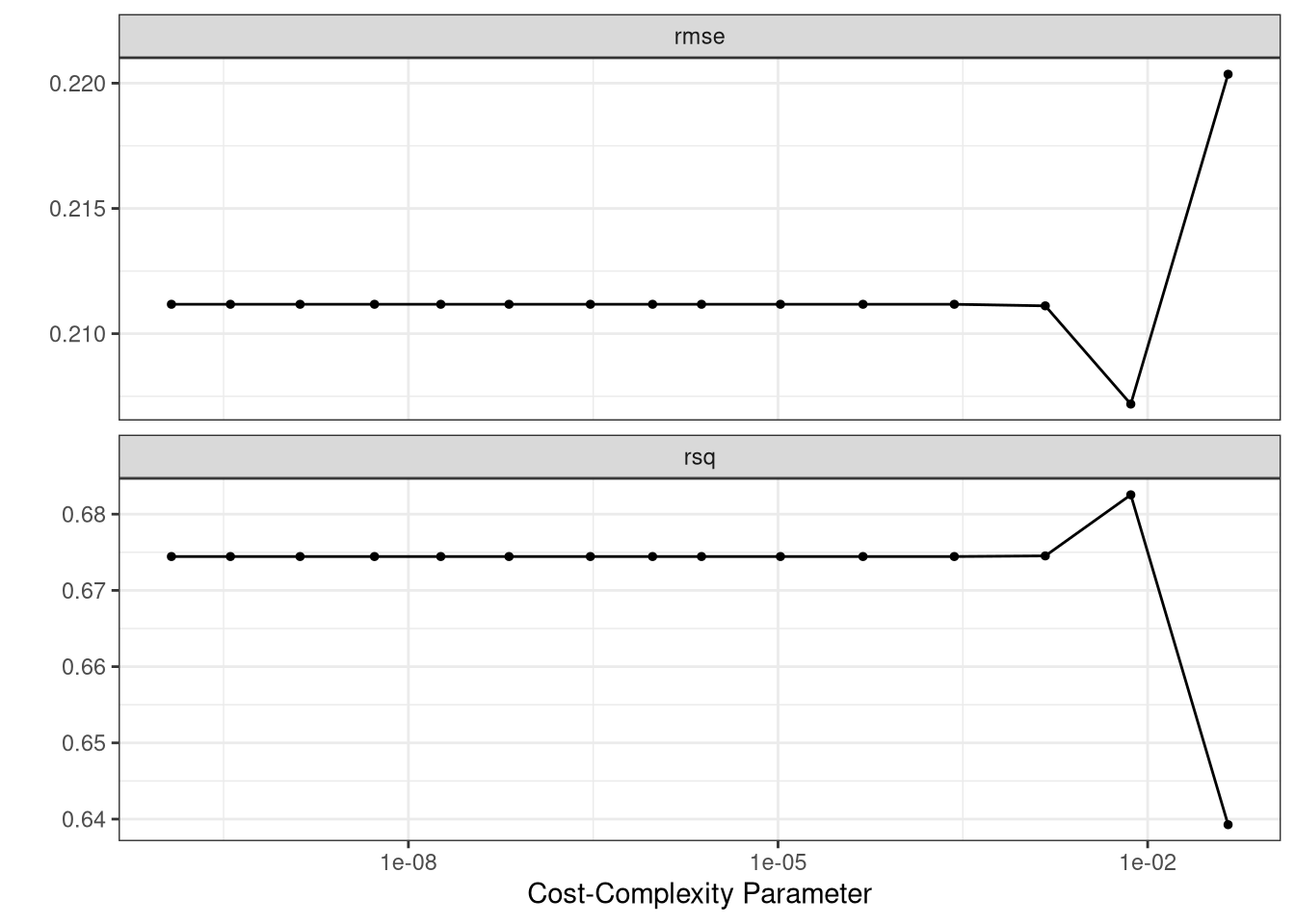
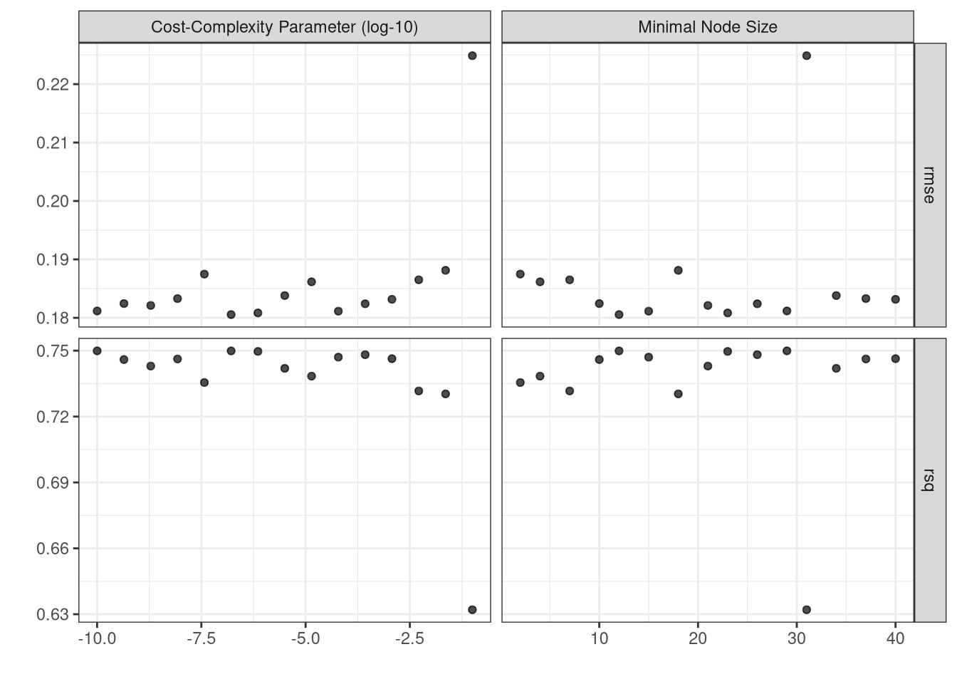
We used 10 fold cross validation repeated 5 times to determine the best value of \(\alpha = 0.0072956\) (cost_complexity) based on the model with the smallest \(RMSE\) (0.2071888). Then we created the final model (final_tree_fit) using cost complexity pruning and show the model in Figure 3.

final_tree_fit |> 
  extract_fit_engine() |> 
  rpart.plot::rpart.plot(roundint = FALSE)

Figure 3: Final tree model after tuning the cost complexity parameter
vip::vip(final_tree_fit) + 
  theme_bw()

Evaluating the Perfomance of your Final Tuned Model on the Test set

augment(final_tree_fit, new_data = hitters_test) |> 
  metrics(truth = salary, estimate = .pred) -> R2
R2 |> 
  knitr::kable()
.metric .estimator .estimate
rmse standard 0.2871821
rsq standard 0.5387941
mae standard 0.1844385
augment(final_tree_fit, new_data = hitters_test) |> 
  ggplot(aes(x = salary, y = .pred)) + 
  geom_abline(lty = "dashed") + 
  geom_smooth(method = "gam", se = FALSE) +
  coord_obs_pred() + 
  geom_point(alpha = 0.5) +
  theme_bw() + 
  labs(x = "Salary (log10) dollars",
       y = "Predicted Salary (log10) dollars",
       title = "R-squared Plot")

library(probably)
augment(final_tree_fit, new_data = hitters_test) |>
cal_plot_regression(truth = salary, estimate = .pred) + 
  theme_bw()

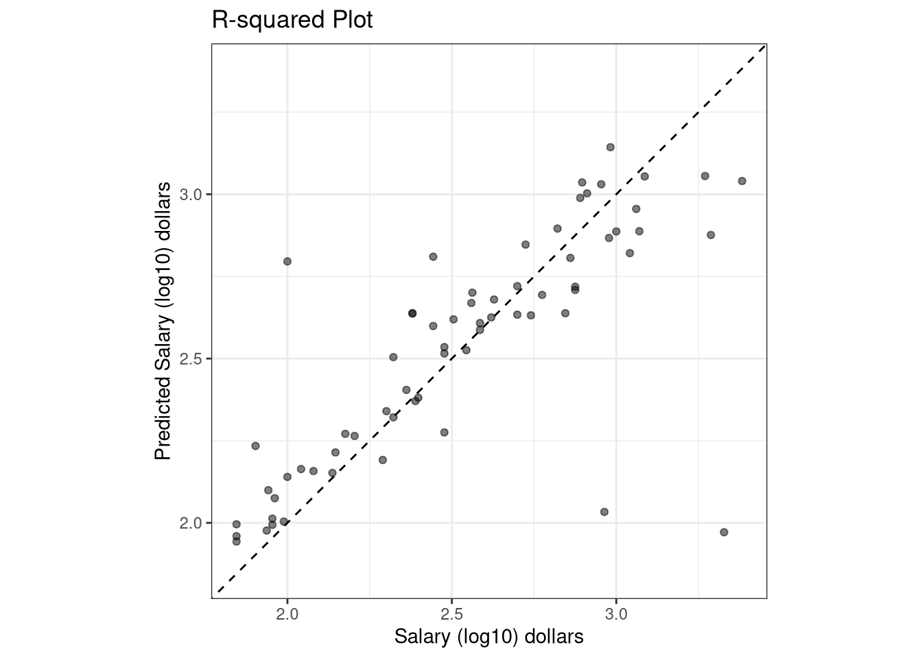
Unfortunately, the model does not perform that well on the test set. The final tuned model has an \(RMSE\) value of $1,937.23, an \(R^2\) value of 53.88% and a mean absolute error of $1,529.11.

Bagging

Decision trees suffer from high variance. This means that if we split the training data into two parts at random, and fit a decision tree to both halves, the results that we get could be quite different. In contrast, a procedure with low variance will yield similar results if applied repeatedly to distinct data sets; linear regression tends to have low variance, if the ratio of \(n\) to \(p\) is moderately large. Bootstrap aggregation, or bagging, is a general-purpose procedure for reducing the variance of a statistical learning method; we introduce it here because it is particularly useful and frequently used in the context of decision trees.

library(baguette)
bag_spec <-
  bag_tree(cost_complexity = tune(), min_n = tune())  |> 
  set_engine('rpart')  |> 
  set_mode('regression')
bag_recipe <- recipe(formula = salary ~ ., data = hitters_train) 
bag_wkfl <- workflow() |> 
  add_recipe(bag_recipe) |> 
  add_model(bag_spec)
bag_wkfl
══ Workflow ════════════════════════════════════════════════════════════════════
Preprocessor: Recipe
Model: bag_tree()

── Preprocessor ────────────────────────────────────────────────────────────────
0 Recipe Steps

── Model ───────────────────────────────────────────────────────────────────────
Bagged Decision Tree Model Specification (regression)

Main Arguments:
  cost_complexity = tune()
  min_n = tune()

Computational engine: rpart 
set.seed(8675)
bag_tune <-
  tune_grid(bag_wkfl, resamples = hitters_folds, grid = 15)
bag_tune
# Tuning results
# 10-fold cross-validation repeated 5 times 
# A tibble: 50 × 5
   splits           id      id2    .metrics          .notes          
   <list>           <chr>   <chr>  <list>            <list>          
 1 <split [177/20]> Repeat1 Fold01 <tibble [30 × 6]> <tibble [0 × 3]>
 2 <split [177/20]> Repeat1 Fold02 <tibble [30 × 6]> <tibble [0 × 3]>
 3 <split [177/20]> Repeat1 Fold03 <tibble [30 × 6]> <tibble [0 × 3]>
 4 <split [177/20]> Repeat1 Fold04 <tibble [30 × 6]> <tibble [0 × 3]>
 5 <split [177/20]> Repeat1 Fold05 <tibble [30 × 6]> <tibble [0 × 3]>
 6 <split [177/20]> Repeat1 Fold06 <tibble [30 × 6]> <tibble [0 × 3]>
 7 <split [177/20]> Repeat1 Fold07 <tibble [30 × 6]> <tibble [0 × 3]>
 8 <split [178/19]> Repeat1 Fold08 <tibble [30 × 6]> <tibble [0 × 3]>
 9 <split [178/19]> Repeat1 Fold09 <tibble [30 × 6]> <tibble [0 × 3]>
10 <split [178/19]> Repeat1 Fold10 <tibble [30 × 6]> <tibble [0 × 3]>
# ℹ 40 more rows
autoplot(bag_tune) + 
  theme_bw()

show_best(bag_tune, metric = "rmse")
# A tibble: 5 × 8
  cost_complexity min_n .metric .estimator  mean     n std_err .config          
            <dbl> <int> <chr>   <chr>      <dbl> <int>   <dbl> <chr>            
1   0.000000164      12 rmse    standard   0.181    50 0.00787 Preprocessor1_Mo…
2   0.000000720      23 rmse    standard   0.181    50 0.00769 Preprocessor1_Mo…
3   0.0000611        15 rmse    standard   0.181    50 0.00806 Preprocessor1_Mo…
4   0.0000000001     29 rmse    standard   0.181    50 0.00754 Preprocessor1_Mo…
5   0.00000000193    21 rmse    standard   0.182    50 0.00771 Preprocessor1_Mo…
bag_param <- select_best(bag_tune, metric = "rmse")
# bag_param <- tibble(cost_complexity = 0.002470553, min_n = 28)
final_bag_wkfl <- bag_wkfl |> 
  finalize_workflow(bag_param)
final_bag_wkfl 
══ Workflow ════════════════════════════════════════════════════════════════════
Preprocessor: Recipe
Model: bag_tree()

── Preprocessor ────────────────────────────────────────────────────────────────
0 Recipe Steps

── Model ───────────────────────────────────────────────────────────────────────
Bagged Decision Tree Model Specification (regression)

Main Arguments:
  cost_complexity = 1.63789370695406e-07
  min_n = 12

Computational engine: rpart 
final_bag_fit <- final_bag_wkfl |> 
  fit(hitters_train)
final_bag_fit
══ Workflow [trained] ══════════════════════════════════════════════════════════
Preprocessor: Recipe
Model: bag_tree()

── Preprocessor ────────────────────────────────────────────────────────────────
0 Recipe Steps

── Model ───────────────────────────────────────────────────────────────────────
Bagged CART (regression with 11 members)

Variable importance scores include:

# A tibble: 19 × 4
   term         value std.error  used
   <chr>        <dbl>     <dbl> <int>
 1 c_at_bat   19.2       0.571     11
 2 c_runs     19.2       0.655     11
 3 c_hits     18.9       0.579     11
 4 crbi       16.5       0.526     11
 5 c_walks    15.5       0.609     11
 6 years      10.4       1.03      11
 7 c_hm_run    3.29      1.43      11
 8 at_bat      2.61      0.277     11
 9 hits        2.49      0.254     11
10 runs        2.28      0.208     11
11 rbi         2.00      0.206     11
12 put_outs    1.47      0.285     11
13 hm_run      1.06      0.179     11
14 walks       0.955     0.145     11
15 assists     0.718     0.231     11
16 errors      0.540     0.0919    11
17 new_league  0.314     0.118      9
18 league      0.274     0.0981     8
19 division    0.0372    0.0144     6

Plotting the variable importance from bagging

final_bag_fit |> extract_fit_engine() -> BFL
BFL$imp 
# A tibble: 19 × 4
   term         value std.error  used
   <chr>        <dbl>     <dbl> <int>
 1 c_at_bat   19.2       0.571     11
 2 c_runs     19.2       0.655     11
 3 c_hits     18.9       0.579     11
 4 crbi       16.5       0.526     11
 5 c_walks    15.5       0.609     11
 6 years      10.4       1.03      11
 7 c_hm_run    3.29      1.43      11
 8 at_bat      2.61      0.277     11
 9 hits        2.49      0.254     11
10 runs        2.28      0.208     11
11 rbi         2.00      0.206     11
12 put_outs    1.47      0.285     11
13 hm_run      1.06      0.179     11
14 walks       0.955     0.145     11
15 assists     0.718     0.231     11
16 errors      0.540     0.0919    11
17 new_league  0.314     0.118      9
18 league      0.274     0.0981     8
19 division    0.0372    0.0144     6
BFL$imp[1:10, ] |> 
  mutate(term = fct_reorder(term, value)) |> 
  ggplot(aes(x = term, y = value)) + 
  geom_col() + 
  coord_flip() + 
  theme_bw()

Evaluating the Perfomance of your Final Tuned Model on the Test set

augment(final_bag_fit, new_data = hitters_test) |> 
  metrics(truth = salary, estimate = .pred) -> R3
R3 |> 
  knitr::kable()
.metric .estimator .estimate
rmse standard 0.2870749
rsq standard 0.5419787
mae standard 0.1717095
augment(final_bag_fit, new_data = hitters_test) |> 
  ggplot(aes(x = salary, y = .pred)) + 
  geom_abline(lty = "dashed") + 
  coord_obs_pred() + 
  geom_point(alpha = 0.5) +
  theme_bw() + 
  labs(x = "Salary (log10) dollars",
       y = "Predicted Salary (log10) dollars",
       title = "R-squared Plot")

The bagged model is an improvement over the decision tree model since the \(RMSE\) decreased to $1,936.76, the \(R^2\) value increased to 54.2%, and the mean absolute error decreased to $1,484.94. Recall that the final tuned single decision tree an \(RMSE\) value of $1,937.23, an \(R^2\) value of 53.88% and a mean absolute error of $1,529.11.

While bagging can improve predictions for many regression methods, it is particularly useful for decision trees. To apply bagging to regression trees, we simply construct \(B\) regression trees using \(B\) bootstrapped training sets, and average the resulting predictions. Each individual tree has high variance, but low bias. Averaging these \(B\) trees reduces the variance. Bagging has been demonstrated to give impressive improvements in accuracy by combining together hundreds or even thousands of trees into a single procedure.

Random Forests

Random forests provide an improvement over bagged trees by way of a small tweak that decorrelates the trees. As in bagging, we build a number of decision trees on bootstrapped training samples. But when building these decision trees, each time a split in a tree is considered, a random sample of \(m\) predictors is chosen as split candidates from the full set of \(p\) predictors. The split is allowed to use only one of those \(m\) predictors. A fresh sample of \(m\) predictors is taken at each split, and typically we choose \(m = \sqrt{p}\) for classification problems and \(p/3\) for regression problems—that is, the number of predictors considered at each split is approximately equal to the square root of the total number of predictors for classification problems or the number of predictors is roughly \(p/3\) at each split for regression problems.

In other words, in building a random forest, at each split in the tree, the algorithm is not even allowed to consider a majority of the available predictors. This may sound crazy, but it has a clever rationale. Suppose that there is one very strong predictor in the data set, along with a number of other moderately strong predictors. Then in the collection of bagged trees, most or all of the trees will use this strong predictor in the top split. Consequently, all of the bagged trees will look quite similar to each other. Hence the predictions from the bagged trees will be highly correlated. Unfortunately, averaging many highly correlated trees does not lead to as large of a reduction in variance as averaging many uncorrelated quantities. In particular, this means that bagging will not lead to a substantial reduction in variance over a single tree in this setting.

The random forest algorithm overcomes this problem by forcing each split to consider only a subset of the predictors. There fore, on average \((p-m)/p\) of the splits will not even consider the strong predictor, and so other predictors will have more of a chance. We can think of this process as decorrelating the trees, thereby making the average of the resulting trees less variable and hence more reliable.

ranger_spec <- rand_forest(mtry = tune(), 
                           min_n = tune(), 
                           trees = 500) |>  
  set_mode("regression")  |>  
  set_engine("ranger",
             importance = "impurity")
ranger_spec
Random Forest Model Specification (regression)

Main Arguments:
  mtry = tune()
  trees = 500
  min_n = tune()

Engine-Specific Arguments:
  importance = impurity

Computational engine: ranger 
ranger_recipe <- recipe(formula = salary ~ ., data = hitters_train)

ranger_workflow <- 
  workflow()  |>  
  add_recipe(ranger_recipe)  |>  
  add_model(ranger_spec) 
set.seed(309)
ranger_tune <-
  tune_grid(ranger_workflow, resamples = hitters_folds, grid = 15)
ranger_tune
# Tuning results
# 10-fold cross-validation repeated 5 times 
# A tibble: 50 × 5
   splits           id      id2    .metrics          .notes          
   <list>           <chr>   <chr>  <list>            <list>          
 1 <split [177/20]> Repeat1 Fold01 <tibble [30 × 6]> <tibble [0 × 3]>
 2 <split [177/20]> Repeat1 Fold02 <tibble [30 × 6]> <tibble [0 × 3]>
 3 <split [177/20]> Repeat1 Fold03 <tibble [30 × 6]> <tibble [0 × 3]>
 4 <split [177/20]> Repeat1 Fold04 <tibble [30 × 6]> <tibble [0 × 3]>
 5 <split [177/20]> Repeat1 Fold05 <tibble [30 × 6]> <tibble [0 × 3]>
 6 <split [177/20]> Repeat1 Fold06 <tibble [30 × 6]> <tibble [0 × 3]>
 7 <split [177/20]> Repeat1 Fold07 <tibble [30 × 6]> <tibble [0 × 3]>
 8 <split [178/19]> Repeat1 Fold08 <tibble [30 × 6]> <tibble [0 × 3]>
 9 <split [178/19]> Repeat1 Fold09 <tibble [30 × 6]> <tibble [0 × 3]>
10 <split [178/19]> Repeat1 Fold10 <tibble [30 × 6]> <tibble [0 × 3]>
# ℹ 40 more rows
autoplot(ranger_tune) + 
  theme_bw()

show_best(ranger_tune, metric = "rmse")
# A tibble: 5 × 8
   mtry min_n .metric .estimator  mean     n std_err .config              
  <int> <int> <chr>   <chr>      <dbl> <int>   <dbl> <chr>                
1     6     2 rmse    standard   0.175    50 0.00752 Preprocessor1_Model05
2     2    10 rmse    standard   0.176    50 0.00677 Preprocessor1_Model02
3     3    21 rmse    standard   0.176    50 0.00696 Preprocessor1_Model03
4     7    12 rmse    standard   0.177    50 0.00763 Preprocessor1_Model06
5    11     4 rmse    standard   0.178    50 0.00779 Preprocessor1_Model09
# ranger_param <- tibble(mtry = 4, min_n = 15)
ranger_param <- select_best(ranger_tune, metric = "rmse")
final_ranger_wkfl <- ranger_workflow |> 
  finalize_workflow(ranger_param)
final_ranger_wkfl 
══ Workflow ════════════════════════════════════════════════════════════════════
Preprocessor: Recipe
Model: rand_forest()

── Preprocessor ────────────────────────────────────────────────────────────────
0 Recipe Steps

── Model ───────────────────────────────────────────────────────────────────────
Random Forest Model Specification (regression)

Main Arguments:
  mtry = 6
  trees = 500
  min_n = 2

Engine-Specific Arguments:
  importance = impurity

Computational engine: ranger 
final_ranger_fit <- final_ranger_wkfl |> 
  fit(hitters_train)

Plotting the variable importance

vip::vip(final_ranger_fit) + 
  theme_bw()

Evaluating the Perfomance of your Final Tuned Model on the Test set

augment(final_ranger_fit, new_data = hitters_test) |> 
  metrics(truth = salary, estimate = .pred) -> R4
R4 |> 
  knitr::kable()
.metric .estimator .estimate
rmse standard 0.2698067
rsq standard 0.5850668
mae standard 0.1575600
augment(final_ranger_fit, new_data = hitters_test) |> 
  ggplot(aes(x = salary, y = .pred)) + 
  geom_abline(lty = "dashed") + 
  coord_obs_pred() + 
  geom_point(alpha = 0.5) +
  theme_bw() + 
  labs(x = "Salary (log10) dollars",
       y = "Predicted Salary (log10) dollars",
       title = "R-squared Plot")

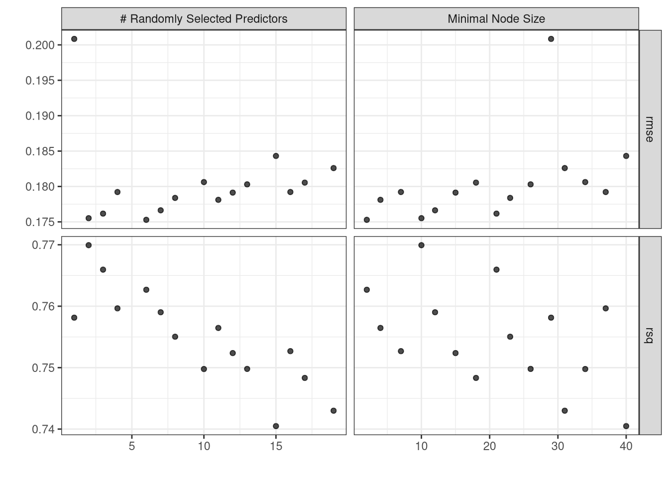
The random forest model is an improvement over the bagged tree model since the \(RMSE\) value decreased to $1,861.26 \(R^2\) value increased to 58.51% and the mean absolute error decreased to $1,437.34. Recall that the final bagged model had an \(RMSE\) of $1,936.76, an \(R^2\) value of 54.2%, and a mean absolute error of $1,484.94.

Boosting

Recall that bagging involves creating multiple copies of the original training data set using the bootstrap, fitting a separate decision tree to each copy, and then combining all of the trees in order to create a single predictive model. Notably, each tree is built on a bootstrap data set, independent of the other trees. Boosting works in a similar way, except that the trees are grown sequentially: each tree is grown using information from previously grown trees. Boosting does not involve bootstrap sampling; instead each tree is fit on a modified version of the original data set.

Like bagging, boosting involves combining a large number of decision trees \(\hat{f}^1,\ldots, \hat{f}^B\).

Boosting for Regression Trees Algorithm
  1. Set \(\hat{f}(x)=0\) and \(r_i = y_i\) for all \(i\) in the training set.

  2. For \(b = 1, 2, \ldots,B\), repeat:

    1. Fit a tree \(\hat{f}^b\) with \(d\) splits (\(d + 1\) terminal nodes) to the training data \((X, r)\).
    2. Update \(\hat{f}\) by adding a shrunken version of the new tree: \[\hat{f}(x) \leftarrow \hat{f}(x) + \lambda \hat{f}^b(x).\]
    3. Update the residuals, \[r_i \leftarrow r_i - \lambda\hat{f}^b(x).\]
  3. Output the boosted model, \[\hat{f}(x) = \sum_{b=1}^{B}\lambda\hat{f}^b(x).\]

What is the idea behind this procedure? Unlike fitting a single large decision tree to the data, which amounts to fitting the data hard and potentially overfitting, the boosting approach instead learns slowly. Given the current model, we fit a decision tree to the residuals from the model. That is, we fit a tree using the current residuals, rather than the outcome \(Y\), as the response. We then add this new decision tree into the fitted function in order to update the residuals. Each of these trees can be rather small, with just a few terminal nodes, determined by the parameter \(d\) in the algorithm. By fitting small trees to the residuals, we slowly improve \(\hat{f}\) in areas where it does not perform well. The shrinkage parameter \(\lambda\) slows the process down even further, allowing more and different shaped trees to attack the residuals. In general, statistical learning approaches that learn slowly tend to perform well. Note that in boosting, unlike in bagging, the construction of each tree depends strongly on the trees that have already been grown.

Boosting Tuning Parameters
  1. The number of trees \(B\). Unlike bagging and random forests, boosting can overfit if \(B\) is too large, although this overfitting tends to occur slowly if at all. We use cross-validation to select \(B\).

  2. The shrinkage parameter \(\lambda\), a small positive number. This controls the rate at which boosting learns. Typical values are 0.01 or 0.001, and the right choice can depend on the problem. Very small \(\lambda\) can require using a very large value of \(B\) in order to achieve good performance.

  3. The number \(d\) of splits in each tree, which controls the complexity of the boosted ensemble. Often \(d = 1\) works well, in which case each tree is a stump, consisting of a single split. In this case, the boosted ensemble is fitting and additive model, since each term involves only a single variable. More generally \(d\) is the interaction depth, and controls the interaction order of the boosted model, since \(d\) splits can involve at most \(d\) variables.

xgboost_spec <- 
  boost_tree(trees = tune(), min_n = tune(), tree_depth = tune(), 
             learn_rate = tune(), loss_reduction = tune(), 
             sample_size = tune()) |>  
  set_mode("regression") |>  
  set_engine("xgboost") 
xgboost_spec
Boosted Tree Model Specification (regression)

Main Arguments:
  trees = tune()
  min_n = tune()
  tree_depth = tune()
  learn_rate = tune()
  loss_reduction = tune()
  sample_size = tune()

Computational engine: xgboost 
xgboost_recipe <- 
  recipe(formula = salary ~  . , data = hitters_train) |>  
  step_normalize(all_numeric_predictors()) |> 
  step_dummy(all_nominal_predictors(), one_hot = TRUE) |> 
  step_zv(all_predictors()) 
xgboost_recipe
xgboost_workflow <- 
  workflow() |>  
  add_recipe(xgboost_recipe) |>  
  add_model(xgboost_spec) 
xgboost_workflow
══ Workflow ════════════════════════════════════════════════════════════════════
Preprocessor: Recipe
Model: boost_tree()

── Preprocessor ────────────────────────────────────────────────────────────────
3 Recipe Steps

• step_normalize()
• step_dummy()
• step_zv()

── Model ───────────────────────────────────────────────────────────────────────
Boosted Tree Model Specification (regression)

Main Arguments:
  trees = tune()
  min_n = tune()
  tree_depth = tune()
  learn_rate = tune()
  loss_reduction = tune()
  sample_size = tune()

Computational engine: xgboost 
set.seed(753)
xgboost_tune <-
  tune_grid(xgboost_workflow, resamples = hitters_folds, grid = 15)
xgboost_tune
# Tuning results
# 10-fold cross-validation repeated 5 times 
# A tibble: 50 × 5
   splits           id      id2    .metrics           .notes          
   <list>           <chr>   <chr>  <list>             <list>          
 1 <split [177/20]> Repeat1 Fold01 <tibble [30 × 10]> <tibble [1 × 3]>
 2 <split [177/20]> Repeat1 Fold02 <tibble [30 × 10]> <tibble [1 × 3]>
 3 <split [177/20]> Repeat1 Fold03 <tibble [30 × 10]> <tibble [1 × 3]>
 4 <split [177/20]> Repeat1 Fold04 <tibble [30 × 10]> <tibble [1 × 3]>
 5 <split [177/20]> Repeat1 Fold05 <tibble [30 × 10]> <tibble [1 × 3]>
 6 <split [177/20]> Repeat1 Fold06 <tibble [30 × 10]> <tibble [1 × 3]>
 7 <split [177/20]> Repeat1 Fold07 <tibble [30 × 10]> <tibble [1 × 3]>
 8 <split [178/19]> Repeat1 Fold08 <tibble [30 × 10]> <tibble [1 × 3]>
 9 <split [178/19]> Repeat1 Fold09 <tibble [30 × 10]> <tibble [1 × 3]>
10 <split [178/19]> Repeat1 Fold10 <tibble [30 × 10]> <tibble [1 × 3]>
# ℹ 40 more rows

There were issues with some computations:

  - Warning(s) x50: A correlation computation is required, but `estimate` is constant...

Run `show_notes(.Last.tune.result)` for more information.

Consider using the finetune package for tuning with the tune_race_anova() function.

set.seed(867)
library(finetune)
doParallel::registerDoParallel()
xgb_tune <- 
  tune_race_anova(xgboost_workflow, resamples = hitters_folds, grid = 15)
xgb_tune
# Tuning results
# 10-fold cross-validation repeated 5 times 
# A tibble: 50 × 6
   splits           id      id2    .order .metrics           .notes          
   <list>           <chr>   <chr>   <int> <list>             <list>          
 1 <split [177/20]> Repeat1 Fold04      3 <tibble [30 × 10]> <tibble [3 × 3]>
 2 <split [177/20]> Repeat1 Fold05      1 <tibble [30 × 10]> <tibble [2 × 3]>
 3 <split [178/19]> Repeat1 Fold08      2 <tibble [30 × 10]> <tibble [3 × 3]>
 4 <split [178/19]> Repeat1 Fold09      4 <tibble [18 × 10]> <tibble [0 × 3]>
 5 <split [177/20]> Repeat1 Fold06      5 <tibble [14 × 10]> <tibble [0 × 3]>
 6 <split [177/20]> Repeat1 Fold01      6 <tibble [10 × 10]> <tibble [0 × 3]>
 7 <split [177/20]> Repeat1 Fold02      7 <tibble [10 × 10]> <tibble [0 × 3]>
 8 <split [177/20]> Repeat1 Fold03      8 <tibble [10 × 10]> <tibble [0 × 3]>
 9 <split [178/19]> Repeat1 Fold10      9 <tibble [10 × 10]> <tibble [0 × 3]>
10 <split [177/20]> Repeat1 Fold07     10 <tibble [8 × 10]>  <tibble [0 × 3]>
# ℹ 40 more rows

There were issues with some computations:

  - Warning(s) x8: A correlation computation is required, but `estimate` is constant...

Run `show_notes(.Last.tune.result)` for more information.
autoplot(xgb_tune) + 
  theme_bw()

show_best(xgb_tune, metric = "rmse")
# A tibble: 5 × 12
  trees min_n tree_depth learn_rate loss_reduction sample_size .metric
  <int> <int>      <int>      <dbl>          <dbl>       <dbl> <chr>  
1   572    15         12    0.210    0.109               0.936 rmse   
2   857    34          8    0.00518  0.00000000439       1     rmse   
3  1714     7         14    0.0405   0.0000000291        0.743 rmse   
4   429    21          4    0.139    0.0000000001        0.614 rmse   
5  1143     4          1    0.0118   0.00247             0.807 rmse   
# ℹ 5 more variables: .estimator <chr>, mean <dbl>, n <int>, std_err <dbl>,
#   .config <chr>
autoplot(xgboost_tune) + 
  theme_bw()

show_best(xgboost_tune, metric = "rmse")
# A tibble: 5 × 12
  trees min_n tree_depth learn_rate loss_reduction sample_size .metric
  <int> <int>      <int>      <dbl>          <dbl>       <dbl> <chr>  
1   572    15         12    0.210         1.09e- 1       0.936 rmse   
2  2000    18          6    0.00343       6.63e-10       0.357 rmse   
3   857    34          8    0.00518       4.39e- 9       1     rmse   
4  1143     4          1    0.0118        2.47e- 3       0.807 rmse   
5  1714     7         14    0.0405        2.91e- 8       0.743 rmse   
# ℹ 5 more variables: .estimator <chr>, mean <dbl>, n <int>, std_err <dbl>,
#   .config <chr>
# xgboost_param <- tibble(trees = 1597, min_n = 12, tree_depth = 6, 
#                         learn_rate = 0.00444 ,loss_reduction = 0.000000282, 
#                        sample_size = 0.651)
xgboost_param <- show_best(xgboost_tune, metric = "rmse")[1, ]
final_xgboost_wkfl <- xgboost_workflow |> 
  finalize_workflow(xgboost_param)
final_xgboost_wkfl 
══ Workflow ════════════════════════════════════════════════════════════════════
Preprocessor: Recipe
Model: boost_tree()

── Preprocessor ────────────────────────────────────────────────────────────────
3 Recipe Steps

• step_normalize()
• step_dummy()
• step_zv()

── Model ───────────────────────────────────────────────────────────────────────
Boosted Tree Model Specification (regression)

Main Arguments:
  trees = 572
  min_n = 15
  tree_depth = 12
  learn_rate = 0.209617999245313
  loss_reduction = 0.10857111194022
  sample_size = 0.935714285714286

Computational engine: xgboost 
final_xgboost_fit <- final_xgboost_wkfl |> 
  fit(hitters_train)

Plotting the variable importance

vip::vip(final_xgboost_fit) +
  theme_bw()

Evaluating the Perfomance of your Final Tuned Model on the Test set

augment(final_xgboost_fit, new_data = hitters_test) |> 
  metrics(truth = salary, estimate = .pred) -> R5
R5 |> 
  knitr::kable()
.metric .estimator .estimate
rmse standard 0.2665800
rsq standard 0.5934309
mae standard 0.1565699
augment(final_xgboost_fit, new_data = hitters_test) |> 
  ggplot(aes(x = salary, y = .pred)) + 
  geom_abline(lty = "dashed") + 
  coord_obs_pred() + 
  geom_point(alpha = 0.5) +
  theme_bw() + 
  labs(x = "Salary (log10) dollars",
       y = "Predicted Salary (log10) dollars",
       title = "R-squared Plot")

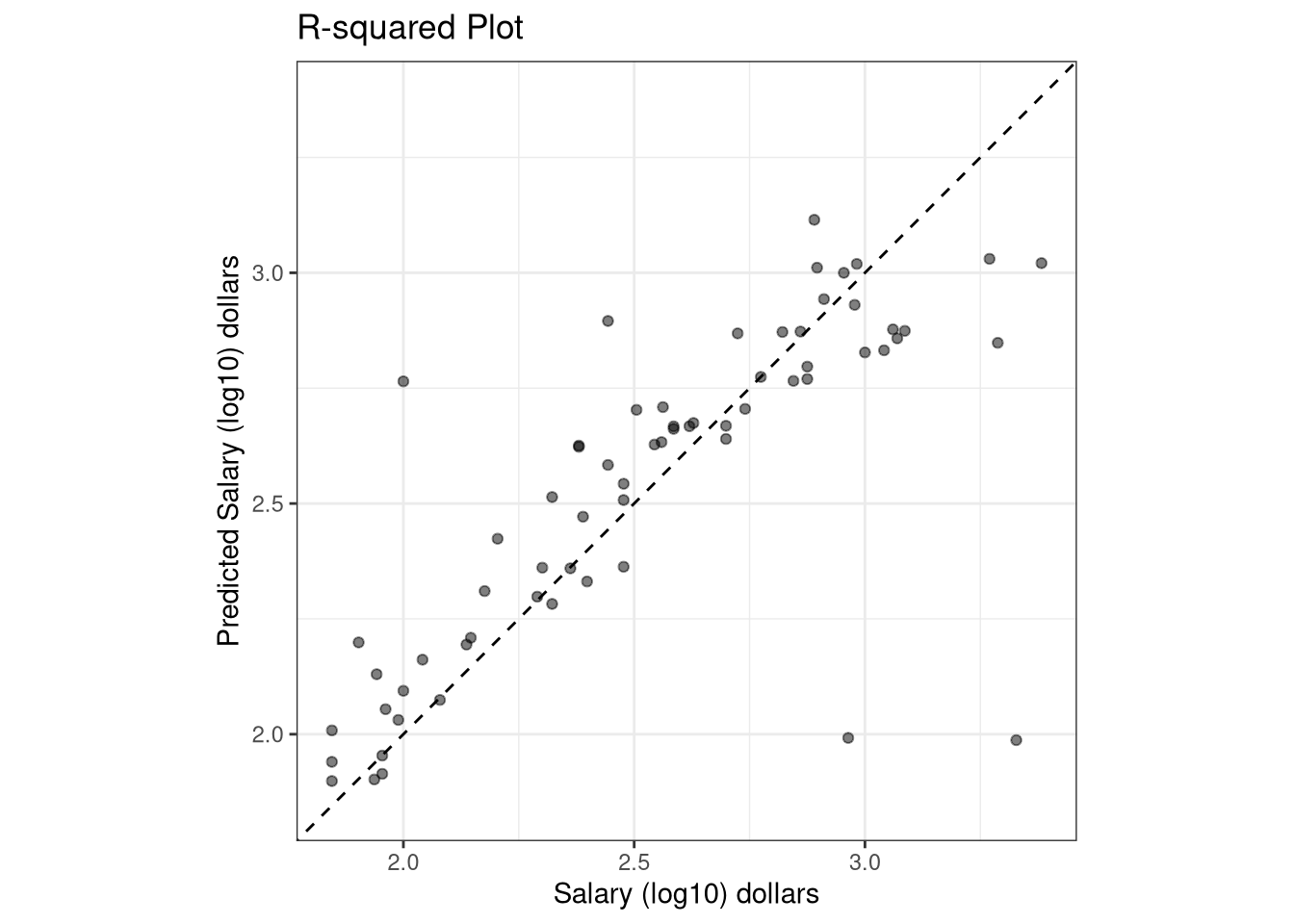
The boosted model is very similar to the random forest model with an \(RMSE\) value of $1,847.48, an \(R^2\) value of 59.34% and a mean absolute error of $1,434.07. Recall that the random forest had an \(RMSE\) value of $1,861.26, an \(R^2\) value of 58.51% and a mean absolute error of $1,437.34.