Chapter 6 Selecting models: a case study in churn prediction
In the final chapter of this course, you’ll learn how to useresamples() to compare multiple models and select (or ensemble) the best one(s).
Reusing a trainControl video
Why reuse a trainControl?
Why reuse a trainControl?
So you can use the same
summaryFunctionand tuning parameters for multiple models.So you don’t have to repeat code when fitting multiple models.
So you can compare models on the exact same training and test data.
All of the above.
6.1 Make custom train/test indices
As you saw in the video, for this chapter you will focus on a real-world dataset that brings together all of the concepts discussed in the previous chapters.
The churn dataset contains data on a variety of telecom customers and the modeling challenge is to predict which customers will cancel their service (or churn).
In this chapter, you will be exploring two different types of predictive models: glmnet and rf, so the first order of business is to create a reusable trainControl object you can use to reliably compare them.
Exercise
churn_x and churn_y are loaded in your workspace.
# library(C50)
# data(churn)
url <- "https://assets.datacamp.com/production/course_1048/datasets/Churn.RData"
download.file(url, "./Data/Churn.RData")
load("./Data/Churn.RData")- Use
createFolds()to create 5 CV folds onchurn_y, your target variable for this exercise.
library(caret)
# Create custom indices: myFolds
myFolds <- createFolds(churn_y, k = 5)- Pass them to
trainControl()to create a reusabletrainControlfor comparing models.
# Create reusable trainControl object: myControl
myControl <- trainControl(
  summaryFunction = twoClassSummary,
  classProbs = TRUE, # IMPORTANT!
  verboseIter = FALSE,
  savePredictions = TRUE,
  index = myFolds
)
Reintroducing glmnet video
glmnet as a baseline model
What makes glmnet a good baseline model?
It’s simple, fast, and easy to interpret.
It always gives poor predictions, so your other models will look good by comparison.
Linear models with penalties on their coefficients always give better results.
6.2 Fit the baseline model
Now that you have a reusable trainControl object called myControl, you can start fitting different predictive models to your churn dataset and evaluate their predictive accuracy.
You’ll start with one of my favorite models, glmnet, which penalizes linear and logistic regression models on the size and number of coefficients to help prevent overfitting.
Exercise
Fit a glmnet model to the churn dataset called model_glmnet. Make sure to use myControl, which you created in the first exercise and is available in your workspace, as the trainControl object.
# Fit glmnet model: model_glmnet
model_glmnet <- train(
  x = churn_x, y = churn_y,
  metric = "ROC",
  method = "glmnet",
  trControl = myControl
)
Reintroducing random forest video
Random forest drawback
What’s the drawback of using a random forest model for churn prediction?
Tree-based models are usually less accurate than linear models.
You no longer have model coefficients to help interpret the model.
Nobody else uses random forests to predict churn.
Note: Random forests are a little bit harder to interpret than linear models, though it is still possible to understand them.
6.3 Random forest with custom trainControl
Another one of my favorite models is the random forest, which combines an ensemble of non-linear decision trees into a highly flexible (and usually quite accurate) model.
Rather than using the classic randomForest package, you’ll be using the ranger package, which is a re-implementation of randomForest that produces almost the exact same results, but is faster, more stable, and uses less memory. I highly recommend it as a starting point for random forest modeling in R.
Exercise
churn_x and churn_y are loaded in your workspace.
Fit a random forest model to the churn dataset. Be sure to use myControl as the trainControl like you’ve done before and implement the "ranger" method.
# Fit random forest: model_rf
model_rf <- train(
  x = churn_x, y = churn_y,
  metric = "ROC",
  method = "ranger",
  trControl = myControl
)
Comparing models video
Matching train/test indices
What’s the primary reason that train/test indices need to match when comparing two models?
You can save a lot of time when fitting your models because you don’t have to remake the datasets.
There’s no real reason; it just makes your plots look better.
Because otherwise you wouldn’t be doing a fair comparison of your models and your results could be due to chance.
Note: Train/test indexes allow you to evaluate your models out of sample so you know that they work!
6.4 Create a resamples object
Now that you have fit two models to the churn dataset, it’s time to compare their out-of-sample predictions and choose which one is the best model for your dataset.
You can compare models in caret using the resamples() function, provided they have the same training data and use the same trainControl object with preset cross-validation folds. resamples() takes as input a list of models and can be used to compare dozens of models at once (though in this case you are only comparing two models).
Exercise
model_glmnet and model_rf are loaded in your workspace.
- Create a
list()containing the glmnet model as item1 and the ranger model as item2.
# Create model_list
model_list <- list(glmnet = model_glmnet, rf = model_rf)- Pass this list to the
resamples()function and save the resulting object asANS.
# Pass model_list to resamples(): ANS
ANS <- resamples(model_list)- Summarize the results by calling
summary()onANS.
# Summarize the results
summary(ANS)
Call:
summary.resamples(object = ANS)

Models: glmnet, rf
Number of resamples: 5

ROC
            Min.   1st Qu.    Median      Mean   3rd Qu.      Max. NA's
glmnet 0.5274094 0.5999116 0.6601143 0.6275889 0.6714286 0.6790805    0
rf     0.7041335 0.7273143 0.7303448 0.7359876 0.7465934 0.7715517    0

Sens
            Min.   1st Qu.    Median      Mean   3rd Qu.      Max. NA's
glmnet 0.9257143 0.9367816 0.9425287 0.9415172 0.9482759 0.9542857    0
rf     0.9828571 0.9885714 0.9942529 0.9931363 1.0000000 1.0000000    0

Spec
             Min.    1st Qu.     Median       Mean    3rd Qu. Max. NA's
glmnet 0.07692308 0.07692308 0.07692308 0.11815385 0.12000000 0.24    0
rf     0.00000000 0.00000000 0.03846154 0.02338462 0.03846154 0.04    0
More on resamples video
6.5 Create a box-and-whisker plot
caret provides a variety of methods to use for comparing models. All of these methods are based on the resamples() function. My favorite is the box-and-whisker plot, which allows you to compare the distribution of predictive accuracy (in this case AUC) for the two models.
In general, you want the model with the higher median AUC, as well as a smaller range between min and max AUC.
You can make this plot using the bwplot() function, which makes a box and whisker plot of the model’s out of sample scores. Box and whisker plots show the median of each distribution as a line and the interquartile range of each distribution as a box around the median line. You can pass the metric = "ROC" argument to the bwplot() function to show a plot of the model’s out-of-sample ROC scores and choose the model with the highest median ROC.
If you do not specify a metric to plot, bwplot() will automatically plot 3 of them.
Exercise
Pass the ANS object to the bwplot() function to make a box-and-whisker plot. Look at the resulting plot and note which model has the higher median ROC statistic. Be sure to specify which metric you want to plot.
# Create bwplot
bwplot(ANS, metric = "ROC")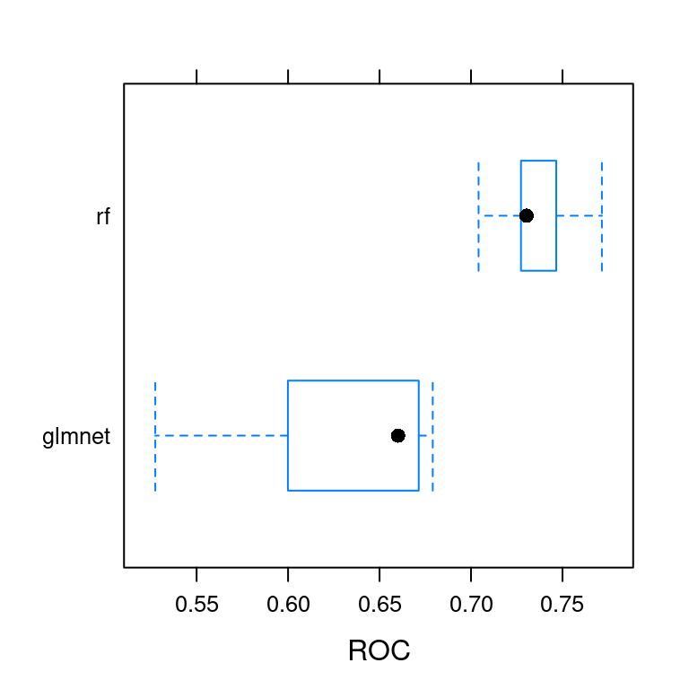
6.6 Create a scatterplot
Another useful plot for comparing models is the scatterplot, also known as the xy-plot. This plot shows you how similar the two models’ performances are on different folds.
It’s particularly useful for identifying if one model is consistently better than the other across all folds, or if there are situations when the inferior model produces better predictions on a particular subset of the data.
Exercise
Pass the ANS object to the xyplot() function. Look at the resulting plot and note how similar the two models’ predictions are (or are not) on the different folds. Be sure to specify which metric you want to plot.
# Create xyplot
xyplot(ANS, metric = "ROC")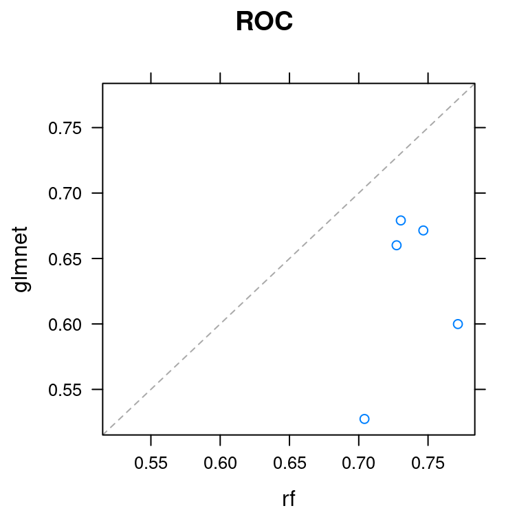
6.7 Ensembling models
That concludes the course! As a teaser for a future course on making ensembles of caret models, I’ll show you how to fit a stacked ensemble of models using the caretEnsemble package.
caretEnsemble provides the caretList() function for creating multiple caret models at once on the same dataset, using the same resampling folds. You can also create your own lists of caret models.
In this exercise, I’ve made a caretList for you, containing the glmnet and ranger models you fit on the churn dataset. Use the caretStack() function to make a stack of caret models, with the two sub-models (glmnet and ranger) feeding into another (hopefully more accurate!) caret model.
Exercise
- Call the
caretStack()function with two arguments,model_listandmethod = "glm", to ensemble the two models using a logistic regression. Store the result asstack.
library(caretEnsemble)
Attaching package: 'caretEnsemble'The following object is masked from 'package:ggplot2':
autoplotmodels <- caretList(
x = churn_x, y = churn_y,
metric = "ROC",
trControl = myControl,
methodList = c("glmnet", "ranger")
)
# Create ensemble model: stack
stack <- caretStack(all.models = models, method = "glm") - Summarize the resulting model with the
summary()function.
summary(stack)
Call:
NULL

Deviance Residuals:
    Min       1Q   Median       3Q      Max
-1.5468  -0.5052  -0.4114  -0.3785   2.4228

Coefficients:
            Estimate Std. Error z value Pr(>|z|)
(Intercept)   2.8438     0.6116   4.650 3.32e-06 ***
glmnet        1.8792     0.6086   3.088  0.00202 **
ranger       -7.3635     1.0814  -6.809 9.80e-12 ***
---
Signif. codes:  0 '***' 0.001 '**' 0.01 '*' 0.05 '.' 0.1 ' ' 1

(Dispersion parameter for binomial family taken to be 1)

    Null deviance: 765.13  on 999  degrees of freedom
Residual deviance: 707.26  on 997  degrees of freedom
AIC: 713.26

Number of Fisher Scoring iterations: 5