Chapter 4 Multiple Regression
This chapter will show you how to add two, three, and even more numeric explanatory variables to a linear model.
4.1 Fitting a MLR model
In terms of the R code, fitting a multiple linear regression model is easy: simply add variables to the model formula you specify in the lm() command.
In a parallel slopes model, we had two explanatory variables: one was numeric and one was categorical. Here, we will allow both explanatory variables to be numeric.
load("./Data/mario_kart.RData")
str(mario_kart)
tibble [141 × 12] (S3: tbl_df/tbl/data.frame)
$ id : num [1:141] 1.5e+11 2.6e+11 3.2e+11 2.8e+11 1.7e+11 ...
$ duration : int [1:141] 3 7 3 3 1 3 1 1 3 7 ...
$ n_bids : int [1:141] 20 13 16 18 20 19 13 15 29 8 ...
$ cond : Factor w/ 2 levels "new","used": 1 2 1 1 1 1 2 1 2 2 ...
$ start_pr : num [1:141] 0.99 0.99 0.99 0.99 0.01 ...
$ ship_pr : num [1:141] 4 3.99 3.5 0 0 4 0 2.99 4 4 ...
$ total_pr : num [1:141] 51.5 37 45.5 44 71 ...
$ ship_sp : Factor w/ 8 levels "firstClass","media",..: 6 1 1 6 2 6 6 8 5 1 ...
$ seller_rate: int [1:141] 1580 365 998 7 820 270144 7284 4858 27 201 ...
$ stock_photo: Factor w/ 2 levels "no","yes": 2 2 1 2 2 2 2 2 2 1 ...
$ wheels : int [1:141] 1 1 1 1 2 0 0 2 1 1 ...
$ title : Factor w/ 80 levels " Mario Kart Wii with Wii Wheel for Wii (New)",..: 80 60 22 7 4 19 34 5 79 70 ...The dataset mario_kart is already loaded in your workspace.
- Fit a multiple linear regression model for total price as a function of the duration of the auction and the starting price.
# Fit the model using duration and start_pr
mod <- lm(total_pr ~ duration + start_pr, data = mario_kart)
mod
Call:
lm(formula = total_pr ~ duration + start_pr, data = mario_kart)

Coefficients:
(Intercept)     duration     start_pr
     51.030       -1.508        0.233
4.2 Tiling the plane
One method for visualizing a multiple linear regression model is to create a heatmap of the fitted values in the plane defined by the two explanatory variables. This heatmap will illustrate how the model output changes over different combinations of the explanatory variables.
This is a multistep process:
- First, create a grid of the possible pairs of values of the explanatory variables. The grid should be over the actual range of the data present in each variable. We’ve done this for you and stored the result as a data frame called
grid.
grid <- expand.grid(duration = seq(1, 10, by = 1), start_pr = seq(0.01, 69.95, by = 0.01))Use
augment()with thenewdataargument to find the \(\hat{y}\)’s corresponding to the values ingrid.Add these to the
data_spaceplot by using the fill aesthetic andgeom_tile().
data_space <- ggplot(data = mario_kart,
                     aes(x = duration, y = start_pr)) +
  geom_point(aes(color = total_pr)) +
  theme_bw()
data_space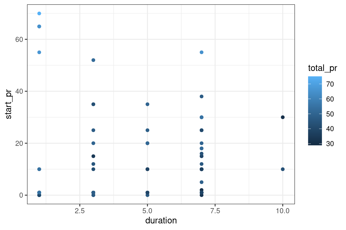
Exercise
The model object mod is already in your workspace.
- Use
augment()to create adata.framethat contains the values the model outputs for each row ofgrid.
# add predictions to grid
price_hats <- broom::augment(mod, newdata = grid)- Use
geom_tileto illustrate these predicted values over thedata_spaceplot. Use thefillaesthetic and setalpha = 0.5.
# tile the plane
data_space +
   geom_tile(data = price_hats,
             aes(fill = .fitted), alpha = 0.5)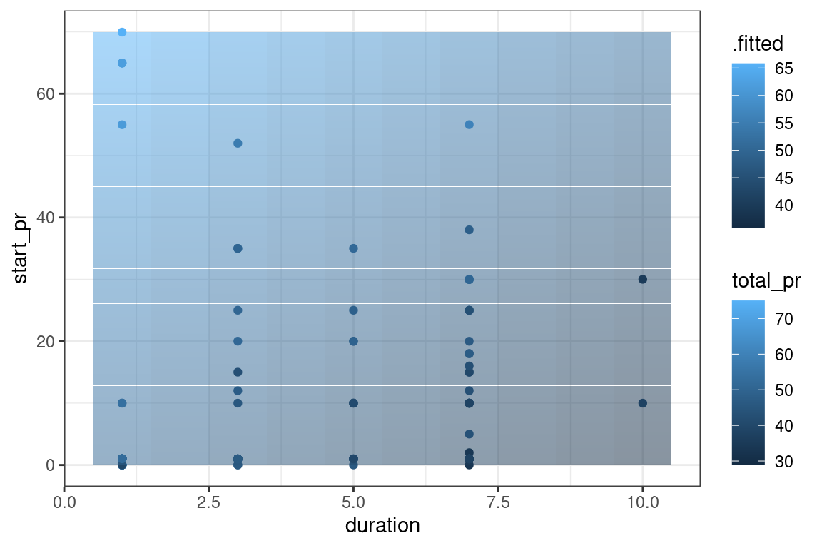
4.3 Models in 3D
An alternative way to visualize a multiple regression model with two numeric explanatory variables is as a plane in three dimensions. This is possible in R using the plotly package.
We have created three objects that you will need:
x: a vector of unique values ofdurationy: a vector of unique values ofstart_prplane: a matrix of the fitted values across all combinations ofxandy
Much like ggplot(), the plot_ly() function will allow you to create a plot object with variables mapped to x, y, and z aesthetics. The add_markers() function is similar to geom_point() in that it allows you to add points to your 3D plot.
Note that plot_ly uses the pipe (%>%) operator to chain commands together.
Exercise
- Run the
plot_lycommand to draw 3D scatterplot fortotal_pras a function of duration andstart_prby mapping thezvariable to the response and thexandyvariables to the explanatory variables. Duration should be on the x-axis and starting price should be on the y-axis.
library(plotly)
# draw the 3D scatterplot
p <- plot_ly(data = mario_kart, z = ~total_pr, x = ~duration, y = ~start_pr, opacity = 0.6) %>%
  add_markers()
p- Use
add_surface()to draw a plane through the cloud of points by settingz = ~plane. See wikipedia for the definition of an outer product. In what follows, we will use the R functionouter()to compute the values ofplane.
\[\bf{u \otimes v} = \bf{uv^T}\]
summary(mod)$coef Estimate Std. Error t value Pr(>|t|)
(Intercept) 51.0295070 1.17913685 43.277001 3.665684e-82
duration -1.5081260 0.25551997 -5.902184 2.644972e-08
start_pr 0.2329542 0.04363644 5.338525 3.755647e-07x <- seq(1, 10, length = 70)
y <- seq(0.010, 59.950, length = 70)
plane <- outer(x, y, function(a, b){summary(mod)$coef[1,1] +
summary(mod)$coef[2,1]*a + summary(mod)$coef[3,1]*b})
# draw the plane
p %>%
add_surface(x = ~x, y = ~y, z = ~plane, showscale = FALSE)Coefficient magnitude
The coefficients from our model for the total auction price of MarioKarts as a function of auction duration and starting price are shown below.
mod
Call:
lm(formula = total_pr ~ duration + start_pr, data = mario_kart)

Coefficients:
(Intercept)     duration     start_pr
     51.030       -1.508        0.233
A colleague claims that these results imply that the duration of the auction is a more important determinant of final price than starting price, because the coefficient is larger. This interpretation is false because:
The coefficient on duration is negative.
Smaller coefficients are more important.
The coefficients have different units (dollars per day and dollars per dollar, respectively) and so they are not directly comparable.
The intercept coefficient is much bigger, so it is the most important one.
Practicing interpretation
Fit a multiple regression model for the total auction price of an item in the mario_kart data set as a function of the starting price and the duration of the auction. Compute the coefficients and choose the correct interpretation of the duration variable.
For each additional day the auction lasts, the expected final price declines by $1.51, after controlling for starting price.
For each additional dollar of starting price, the expected final price increases by $0.23, after controlling for the duration of the auction.
The duration of the auction is a more important determinant of final price than starting price, because the coefficient is larger.
The average auction lasts 51 days.
4.4 Visualizing parallel planes
By including the duration, starting price, and condition variables in our model, we now have two explanatory variables and one categorical variable. Our model now takes the geometric form of two parallel planes!
The first plane corresponds to the model output when the condition of the item is new, while the second plane corresponds to the model output when the condition of the item is used. The planes have the same slopes along both the duration and starting price axes—it is the z-intercept that is different.
Once again we have stored the x and y vectors for you. Since we now have two planes, there are matrix objects plane0 and plane1 stored for you as well.
modI <- lm(total_pr ~ duration + start_pr + cond, data = mario_kart)
summary(modI)$coef
Estimate Std. Error t value Pr(>|t|)
(Intercept) 53.3447530 1.0804915 49.370822 3.781243e-89
duration -0.6559841 0.2553503 -2.568957 1.127073e-02
start_pr 0.1981653 0.0382717 5.177855 7.835882e-07
condused -8.9493214 1.3237851 -6.760403 3.635333e-10plane0 <- outer(x, y, function(a, b){53.3447530 -0.6559841*a +
0.1981653*b})
plane1 <- outer(x, y, function(a, b){53.3447530 -0.6559841*a +
0.1981653*b - 8.9493214})Exercise
- Use
plot_lyto draw 3D scatterplot fortotal_pras a function ofduration,start_pr, andcondby mapping thezvariable to the response and thexandyvariables to the explanatory variables. Duration should be on the x-axis and starting price should be on the y-axis. Use color to representcond.
# draw the 3D scatterplot
p <- plot_ly(data = mario_kart, z = ~total_pr, x = ~duration, y = ~start_pr, opacity = 0.6) %>%
  add_markers(color = ~cond)
p- Use
add_surface()(twice) to draw two planes through the cloud of points, one for new MarioKarts and another for used ones. Use the objectsplane0andplane1.
# draw two planes
p %>%
  add_surface(x = ~x, y = ~y, z = ~plane0, showscale = FALSE) %>%
  add_surface(x = ~x, y = ~y, z = ~plane1, showscale = FALSE)
Parallel plane interpretation
The coefficients from our parallel planes model is shown below.
modI
Call:
lm(formula = total_pr ~ duration + start_pr + cond, data = mario_kart)

Coefficients:
(Intercept)     duration     start_pr     condused
    53.3448      -0.6560       0.1982      -8.9493
Choose the right interpretation of \(\beta_3\) (the coefficient on condUsed):
The expected premium for new (relative to used) MarioKarts is $8.95, after controlling for the duration and starting price of the auction.
The expected premium for used (relative to new) MarioKarts is $8.95, after controlling for the duration and starting price of the auction.
For each additional day the auction lasts, the expected final price declines by $8.95, after controlling for starting price and condition.
Interpretation of coefficient in a big model
This time we have thrown even more variables into our model, including the number of bids in each auction (n_bids) and the number of wheels. Unfortunately this makes a full visualization of our model impossible, but we can still interpret the coefficients.
modJ <- lm(total_pr ~ duration + start_pr + cond + wheels + n_bids,
    data = mario_kart)
modJ
Call:
lm(formula = total_pr ~ duration + start_pr + cond + wheels +
    n_bids, data = mario_kart)

Coefficients:
(Intercept)     duration     start_pr     condused       wheels       n_bids
    39.3741      -0.2752       0.1796      -4.7720       6.7216       0.1909
Choose the correct interpretation of the coefficient on the number of wheels:
The average number of wheels is 6.72.
Each additional wheel costs exactly $6.72.
Each additional wheel is associated with an increase in the expected auction price of $6.72.
Each additional wheel is associated with an increase in the expected auction price of $6.72, after controlling for auction duration, starting price, number of bids, and the condition of the item.